TSP From DP to Deep Learning. Episode 2: DP on Euclidean Dataset

This is second episode of series: TSP From DP to Deep Learning.

• Episode 1: AC TSP on AIZU with recursive DP
• Episode 2: TSP DP on a Euclidean Dataset
• Episode 3: Pointer Networks in PyTorch
• Episode 4: Search for Most Likely Sequence
• Episode 5: Reinforcement Learning PyTorch Implementation

AIZU TSP Bottom Up Iterative DP

In last episode, we provided a top down recursive DP in Python 3 and Java 8. Now we continue to improve and convert it to bottom up iterative DP version. Below is a graph with 3 vertices, the top down recursive calls are completely drawn.

Looking from bottom up, we could identify corresponding topological computing order with ease. First, we compute all bit states with 3 ones, then 2 ones, then 1 one.

Pseudo Java code below.

for (int bitset_num = N; bitset_num >=0; bitset_num++) {
	while(hasNextCombination(bitset_num)) {
		int state = nextCombination(bitset_num);
		// compute dp[state][v], v-th bit is set in state
		for (int v = 0; v < n; v++) {
			for (int u = 0; u < n; u++) {
				// for each u not reached by this state
				if (!include(state, u)) {
					dp[state][v] = min(dp[state][v], 
						dp[new_state_include_u][u] + dist[v][u]);
				}
			}
		}
	}
}

For example, dp[00010][1] is the min distance starting from vertex 0, and just arriving at vertex 1: \(0 \rightarrow 1 \rightarrow ? \rightarrow ? \rightarrow ? \rightarrow 0\). In order to find out total min distance, we need to enumerate all possible u for first question mark. \[ (0 \rightarrow 1) + \begin{align*} \min \left\lbrace \begin{array}{r@{}l} 2 \rightarrow ? \rightarrow ? \rightarrow 0 + dist(1,2) \qquad\text{ new_state=[00110][2] } \qquad\\\\ 3 \rightarrow ? \rightarrow ? \rightarrow 0 + dist(1,3) \qquad\text{ new_state=[01010][3] } \qquad\\\\ 4 \rightarrow ? \rightarrow ? \rightarrow 0 + dist(1,4) \qquad\text{ new_state=[10010][4] } \qquad \end{array} \right. \end{align*} \]

Java Iterative DP Code

AC code in Python 3 and Java 8. Illustrate core Java code below.

{linenos

public long solve() {
	int N = g.V_NUM;
	long[][] dp = new long[1 << N][N];
	// init dp[][] with MAX
	for (int i = 0; i < dp.length; i++) {
		Arrays.fill(dp[i], Integer.MAX_VALUE);
	}
	dp[(1 << N) - 1][0] = 0;

	for (int state = (1 << N) - 2; state >= 0; state--) {
		for (int v = 0; v < N; v++) {
			for (int u = 0; u < N; u++) {
				if (((state >> u) & 1) == 0) {
					dp[state][v] = Math.min(dp[state][v], dp[state | 1 << u][u] + g.edges[v][u]);
				}
			}
		}
	}
	return dp[0][0] == Integer.MAX_VALUE ? -1 : dp[0][0];
}

In this way, runtime complexity can be spotted easily, three for loops leading to O(\(2^n * n * n\)) = O(\(2^n*n^2\) ).

DP on Euclidean Dataset

So far, TSP DP has been crystal clear and we move forward to introducing PTR_NET dataset on Google Drive by Oriol Vinyals who is the author of Pointer Networks. Each line in the dataset has the following pattern:

x0, y0, x1, y1, ... output 1 v1 v2 v3 ... 1

It first lists n points in (x, y) coordinate, followed by "output", then followed by one of the minimal distance tours, starting and ending with vertex 1 (indexed from 1 not 0).

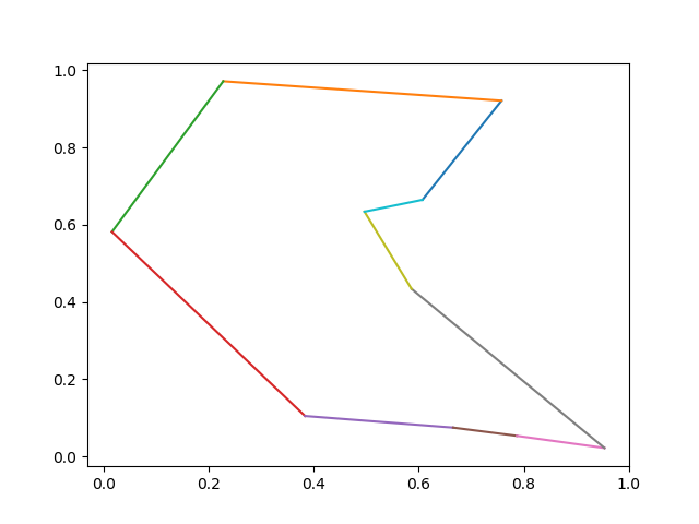
Some examples of 10 vertices are:

0.607122 0.664447 0.953593 0.021519 0.757626 0.921024 0.586376 0.433565 0.786837 0.052959 0.016088 0.581436 0.496714 0.633571 0.227777 0.971433 0.665490 0.074331 0.383556 0.104392 output 1 3 8 6 10 9 5 2 4 7 1 
0.930534 0.747036 0.277412 0.938252 0.794592 0.794285 0.961946 0.261223 0.070796 0.384302 0.097035 0.796306 0.452332 0.412415 0.341413 0.566108 0.247172 0.890329 0.429978 0.232970 output 1 3 2 9 6 5 8 7 10 4 1 
0.686712 0.087942 0.443054 0.277818 0.494769 0.985289 0.559706 0.861138 0.532884 0.351913 0.712561 0.199273 0.554681 0.657214 0.909986 0.277141 0.931064 0.639287 0.398927 0.406909 output 1 5 2 10 7 4 3 9 8 6 1 

Plot first example using code below.

{linenos

import matplotlib.pyplot as plt
points='0.607122 0.664447 0.953593 0.021519 0.757626 0.921024 0.586376 0.433565 0.786837 0.052959 0.016088 0.581436 0.496714 0.633571 0.227777 0.971433 0.665490 0.074331 0.383556 0.104392'
float_list = list(map(lambda x: float(x), points.split(' ')))

x,y = [],[]
for idx, p in enumerate(float_list):
  if idx % 2 == 0:
    x.append(p)
  else:
    y.append(p)

for i in range(0, len(x)):
  for j in range(0, len(x)):
    if i == j:
      continue
    plt.plot((x[i],x[j]),(y[i],y[j]))

plt.show()

TSP Case Fully Connected

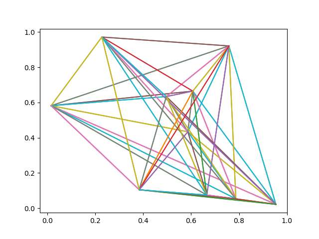
Now plot the optimal tour: \[ 1 \rightarrow 3 \rightarrow 8 \rightarrow 6 \rightarrow 10 \rightarrow 9 \rightarrow 5 \rightarrow 2 \rightarrow 4 \rightarrow 7 \rightarrow 1 \]

{linenos

tour_str = '1 3 8 6 10 9 5 2 4 7 1'
tour = list(map(lambda x: int(x), tour_str.split(' ')))

for i in range(0, len(tour)-1):
  p1 = tour[i] - 1
  p2 = tour[i + 1] - 1
  plt.plot((x[p1],x[p2]),(y[p1],y[p2]))
plt.show()

TSP Case Minimal Tour

Python Code Illustrated

Init Graph Edges

Based on previous top down version, several changes are made. First, we need to have an edge between every 2 vertices and due to our matrix representation of the directed edge, edges of 2 directions are initialized.

{linenos

g: Graph = Graph(N)
for v in range(N):
	for u in range(N):
		diff_x = coordinates[v][0] - coordinates[u][0]
		diff_y = coordinates[v][1] - coordinates[u][1]
		dist: float = math.sqrt(diff_x * diff_x + diff_y * diff_y)
		g.setDist(u, v, dist)
		g.setDist(v, u, dist)

Auxilliary Variable to Track Tour Vertices

One major enhancement is to record the optimal tour during enumerating. We introduce another variable parent[bitstate][v] to track next vertex u, with shortest path.

{linenos

ret: float = FLOAT_INF
u_min: int = -1
	for u in range(self.g.v_num):
		if (state & (1 << u)) == 0:
			s: float = self._recurse(u, state | 1 << u)
				if s + edges[v][u] < ret:
					ret = s + edges[v][u]
					u_min = u
	dp[state][v] = ret
	self.parent[state][v] = u_min

After minimal tour distance is found, one optimal tour is formed with the help of parent variable.

{linenos

def _form_tour(self):
	self.tour = [0]
	bit = 0
	v = 0
	for _ in range(self.g.v_num - 1):
		v = self.parent[bit][v]
		self.tour.append(v)
		bit = bit | (1 << v)
	self.tour.append(0)

Note that for each test case, only one tour is given after "output". Our code may form a different tour but it has same distance as what the dataset generates, which can be verified by following code snippet. See full code on github.

{linenos

tsp: TSPSolver = TSPSolver(g)
tsp.solve()

output_dist: float = 0.0
output_tour = list(map(lambda x: int(x) - 1, output.split(' ')))
for v in range(1, len(output_tour)):
	pre_v = output_tour[v-1]
	curr_v = output_tour[v]
	diff_x = coordinates[pre_v][0] - coordinates[curr_v][0]
	diff_y = coordinates[pre_v][1] - coordinates[curr_v][1]
	dist: float = math.sqrt(diff_x * diff_x + diff_y * diff_y)
	output_dist += dist

	passed = abs(tsp.dist - output_dist) < 10e-5
	if passed:
		print(f'passed dist={tsp.tour}')
	else:
		print(f'Min Tour Distance = {output_dist}, Computed Tour Distance = {tsp.dist}, Expected Tour = {output_tour}, Result = {tsp.tour}')