#Dynamic Programming

This is fourth episode of series: TSP From DP to Deep Learning. In this episode, we systematically compare different searching algorithms for finding most likely sequence in the context of simplied markov chain setting. These models can be further utilized in deep learning decoding stage, which will be illustrated in reinforcement learning, in the next episode. Full list of this series is listed below.

Problem as Markov Chain

In sequence-to-sequence problem, we are always faced with same problem of determining the best or most likely sequence of output. This kind of recurring problem exists extensively in algorithms, machine learning where we are given initial states and the dynamics of the system, and the goal is to find a path that is most likely. The corresponding concept, in science or mathematical discipline, is called Markov Chain.

Let describe the problem in the context of markov chain. Suppose there are \(n\) states, and initial state is given by $s_0 = [0.35, 0.25, 0.4] $. The transition matrix is defined by \(T\) where $ T[i][j]$ denotes the probability of transitioning from \(i\) to \(j\). Notice that each row sums to \(1.0\). \[ T= \begin{matrix} & \begin{matrix}0&1&2\end{matrix} \\\\ \begin{matrix}0\\\\1\\\\2\end{matrix} & \begin{bmatrix}0.3&0.6&0.1\\\\0.4&0.2&0.4\\\\0.3&0.3&0.4\end{bmatrix}\\\\ \end{matrix} \]

Probability of the next state \(s_1\) is derived by multiplication of \(s_0\) and \(T\), which can be visually interpreted by animation below.

The actual probability distribution value of \(s_1\) is computed numerically below. Recall that left multiplying a row with a matrix amounts to making a linear combination of that row vector.

\[ s_1 = \begin{bmatrix}0.35& 0.25& 0.4\end{bmatrix} \begin{matrix} \begin{bmatrix}0.3&0.6&0.1\\\\0.4&0.2&0.4\\\\0.3&0.3&0.4\end{bmatrix}\\\\ \end{matrix} = \begin{bmatrix}0.325& 0.35& 0.255\end{bmatrix} \] Again, state \(s_2\) can be derived in the same way \(s_1 \times T\), where we assume the transitioning dynamics remains the same. However, in deep learning problem, the dynamics usually depends on \(s_i\), or vary according to the stage.

Suppose there are only 3 stages in our problem, e.g., \(s_0 \rightarrow s_1 \rightarrow s_2\). Let \(L\) be the number of stages and \(N\) be the number of vertices in each stage. Hence \(L=N=3\) in our problem setting. There could be \(N^L\) different paths starting from initial stage and to final stage.

Let us compute an arbitrary path probability as an example, \(2(s_0) \rightarrow 1(s_1) \rightarrow 2(s_2)\). The total probability is

\[ p(2 \rightarrow 1 \rightarrow 2) = s_0[2] \times T[2][1] \times T[1][2] = 0.4 \times 0.3 \times 0.4 = 0.048 \]

First, we implement \(N^L\) exhaustive or brute force search.

The following Python 3 function returns one most likely sequence and its probability. Running the algorithm with our example produces 0.084 and route \(0 \rightarrow 1 \rightarrow 2\).

{linenos
1
2
3
4
5
6
7
8
9
10
11
12
13
14
15
16
17
18
19
def search_brute_force(initial: List, transition: List, L: int) -> Tuple[float, Tuple]:
from itertools import combinations_with_replacement
v = [0, 1, 2]
path_all = combinations_with_replacement(v, L)

max_prop = 0.0
max_route = None
prob = 0.0
for path in list(path_all):
for idx, v in enumerate(path):
if idx == 0:
prob = initial[v] # reset to initial state
else:
prev_v = path[idx-1]
prob *= transition[prev_v][v]
if prob > max_prop:
max_prop = max(max_prop, prob)
max_route = path
return max_prop, max_route

Exhaustive search always generates most likely sequence, as searching for a needle in the hay at the cost of exponential runtime complexity \(O(N^L)\). The simplest strategy, unknown as greedy, identifies one vertex in each stage and then expand the vertex in next stage. This strategy, of course, is not guaranteed to find most likely sequence but is fast. See animation below.

Code in Python 3 is given below. Numpy package is employed to utilize np.argmax() for code clarity. Notice there are 2 for loops (the other is np.argmax) so the runtime complexity is \(O(N\times L)\).

{linenos
1
2
3
4
5
6
7
8
9
10
11
12
13
14
15
16
17
18
def search_greedy(initial: List, transition: List, L: int) -> Tuple[float, Tuple]:
import numpy as np
max_route = []
max_prop = 0.0
states = np.array(initial)

prev_max_v = None
for l in range(0, L):
max_v = np.argmax(states)
max_route.append(max_v)
if l == 0:
max_prop = initial[max_v]
else:
max_prop = max_prop * transition[prev_max_v][max_v]
states = max_prop * states
prev_max_v = max_v

return max_prop, max_route

We could improve greedy strategy a little bit by expanding more vertices in each stage. In beam search with \(k\) nodes, the strategy is in each stage, identify \(k\) nodes with highest probability and expand these \(k\) nodes into next stage. In our example, \(k=2\), we select first 2 nodes in stage \(s_0\), expand these 2 nodes and evaluate \(2 \times 3\) nodes in stage \(s_1\), then select 2 nodes and evaluate 6 nodes in stage \(s_2\). Beam search, similar to greedy strategy, is not guaranteed to find most likely sequence but it extends search space with linear complexity.

Below is implementation in Python 3 with PriorityQueue to select top \(k\) nodes. Notice in order to use reverse order of PriorityQueue, a class with @total_ordering is required to be defined. The runtime complexity is \(O(k\times N \times L)\) .

{linenos
1
2
3
4
5
6
7
8
9
10
11
12
13
14
15
16
17
18
19
20
21
22
23
24
25
26
27
28
29
30
31
32
33
34
35
36
37
38
def search_beam(initial: List, transition: List, L: int, K: int) -> Tuple[float, Tuple]:
N = len(initial)
from queue import PriorityQueue
current_q = PriorityQueue()
next_q = PriorityQueue()

from functools import total_ordering
@total_ordering
class PQItem(object):
def __init__(self, prob, route):
self.prob = prob
self.route = route
self.last_v = int(route[-1])

def __eq__(self, other):
return self.prob == other.prob

def __lt__(self, other):
return self.prob > other.prob

for v in range(N):
next_q.put(PQItem(initial[v], str(v)))

for l in range(1, L):
current_q = next_q
next_q = PriorityQueue()
k = K
while not current_q.empty() and k > 0:
item = current_q.get()
prob, route, prev_v = item.prob, item.route, item.last_v
k -= 1
for v in range(N):
nextItem = PQItem(prob * transition[prev_v][v], route + str(v))
next_q.put(nextItem)

max_item = next_q.get()

return max_item.prob, list(map(lambda x: int(x), max_item.route))

Viterbi DP

Similarly to TSP DP version, there is a dynamic programming approach, widely known as Viterbi algorithm, that always finds out sequence with max probability while reducing runtime complexity from \(O(N^L)\) to \(O(L \times N \times N)\) (corresponding to 3 loops in code below). The core idea is in each stage, an array keeps most likely sequence ending with each vertex and use the dp array as input to next stage. For example, let \(dp[1][0]\) be the most likely probability in \(s_1\) stage and end with vertex 0. \[ dp[1][0] = \max \\{s_0[0] \rightarrow s_1[0], s_0[1] \rightarrow s_1[0], s_0[2] \rightarrow s_1[0]\\} \]

Illustrative code that returns max probability but not route, in order to emphasize 3 loop pattern and max operation, honoring the essence of the algorithm.

{linenos
1
2
3
4
5
6
7
8
9
10
11
def search_dp(initial: List, transition: List, L: int) -> float:
N = len(initial)
dp = [[0.0 for c in range(N)] for r in range(L)]
dp[0] = initial[:]

for l in range(1, L):
for v in range(N):
for prev_v in range(N):
dp[l][v] = max(dp[l][v], dp[l - 1][prev_v] * transition[prev_v][v])

return max(dp[L-1])

Probabilistic Sampling

All algorithms described above are deterministic. However, in NLP deep learning decoding, deterministic property has disadvantage in that it may get trapped into repeated phrases or sentences. For example, paragraph like below is commonly generated:

1
This is the best of best of best of ...
One way to get out of loop is resorting to probabilistic sampling. For example, we can generate one vertex in each stage probabilistically according to their weights or according to total path probability.

For demonstration purpose, here is the code based on greedy strategy which probabilistically determines one node at each stage.

{linenos
1
2
3
4
5
6
7
8
9
10
11
12
13
14
15
16
def search_prob_greedy(initial: List, transition: List, L: int) -> Tuple[float, Tuple]:
import random
N = len(initial)
max_route = []
max_prop = 0.0
vertices = [i for i in range(N)]
prob = initial[:]

for l in range(0, L):
v_lst = random.choices(vertices, prob)
v = v_lst[0]
max_route.append(v)
max_prop = prob[v]
prob = [prob[v] * transition[v][v_target] for v_target in range(N)]

return max_prop, max_route

This is second episode of series: TSP From DP to Deep Learning.

AIZU TSP Bottom Up Iterative DP

In last episode, we provided a top down recursive DP in Python 3 and Java 8. Now we continue to improve and convert it to bottom up iterative DP version. Below is a graph with 3 vertices, the top down recursive calls are completely drawn.

Looking from bottom up, we could identify corresponding topological computing order with ease. First, we compute all bit states with 3 ones, then 2 ones, then 1 one.

Pseudo Java code below.

1
2
3
4
5
6
7
8
9
10
11
12
13
14
15
16
for (int bitset_num = N; bitset_num >=0; bitset_num++) {
while(hasNextCombination(bitset_num)) {
int state = nextCombination(bitset_num);
// compute dp[state][v], v-th bit is set in state
for (int v = 0; v < n; v++) {
for (int u = 0; u < n; u++) {
// for each u not reached by this state
if (!include(state, u)) {
dp[state][v] = min(dp[state][v],
dp[new_state_include_u][u] + dist[v][u]);
}
}
}
}
}

For example, dp[00010][1] is the min distance starting from vertex 0, and just arriving at vertex 1: \(0 \rightarrow 1 \rightarrow ? \rightarrow ? \rightarrow ? \rightarrow 0\). In order to find out total min distance, we need to enumerate all possible u for first question mark. \[ (0 \rightarrow 1) + \begin{align*} \min \left\lbrace \begin{array}{r@{}l} 2 \rightarrow ? \rightarrow ? \rightarrow 0 + dist(1,2) \qquad\text{ new_state=[00110][2] } \qquad\\\\ 3 \rightarrow ? \rightarrow ? \rightarrow 0 + dist(1,3) \qquad\text{ new_state=[01010][3] } \qquad\\\\ 4 \rightarrow ? \rightarrow ? \rightarrow 0 + dist(1,4) \qquad\text{ new_state=[10010][4] } \qquad \end{array} \right. \end{align*} \]

Java Iterative DP Code

AC code in Python 3 and Java 8. Illustrate core Java code below.

{linenos
1
2
3
4
5
6
7
8
9
10
11
12
13
14
15
16
17
18
19
20
public long solve() {
int N = g.V_NUM;
long[][] dp = new long[1 << N][N];
// init dp[][] with MAX
for (int i = 0; i < dp.length; i++) {
Arrays.fill(dp[i], Integer.MAX_VALUE);
}
dp[(1 << N) - 1][0] = 0;

for (int state = (1 << N) - 2; state >= 0; state--) {
for (int v = 0; v < N; v++) {
for (int u = 0; u < N; u++) {
if (((state >> u) & 1) == 0) {
dp[state][v] = Math.min(dp[state][v], dp[state | 1 << u][u] + g.edges[v][u]);
}
}
}
}
return dp[0][0] == Integer.MAX_VALUE ? -1 : dp[0][0];
}

In this way, runtime complexity can be spotted easily, three for loops leading to O(\(2^n * n * n\)) = O(\(2^n*n^2\) ).

DP on Euclidean Dataset

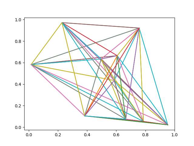
So far, TSP DP has been crystal clear and we move forward to introducing PTR_NET dataset on Google Drive by Oriol Vinyals who is the author of Pointer Networks. Each line in the dataset has the following pattern:

1
x0, y0, x1, y1, ... output 1 v1 v2 v3 ... 1

It first lists n points in (x, y) coordinate, followed by "output", then followed by one of the minimal distance tours, starting and ending with vertex 1 (indexed from 1 not 0).

Some examples of 10 vertices are:

1
2
3
4
0.607122 0.664447 0.953593 0.021519 0.757626 0.921024 0.586376 0.433565 0.786837 0.052959 0.016088 0.581436 0.496714 0.633571 0.227777 0.971433 0.665490 0.074331 0.383556 0.104392 output 1 3 8 6 10 9 5 2 4 7 1 
0.930534 0.747036 0.277412 0.938252 0.794592 0.794285 0.961946 0.261223 0.070796 0.384302 0.097035 0.796306 0.452332 0.412415 0.341413 0.566108 0.247172 0.890329 0.429978 0.232970 output 1 3 2 9 6 5 8 7 10 4 1
0.686712 0.087942 0.443054 0.277818 0.494769 0.985289 0.559706 0.861138 0.532884 0.351913 0.712561 0.199273 0.554681 0.657214 0.909986 0.277141 0.931064 0.639287 0.398927 0.406909 output 1 5 2 10 7 4 3 9 8 6 1

Plot first example using code below.

{linenos
1
2
3
4
5
6
7
8
9
10
11
12
13
14
15
16
17
18
import matplotlib.pyplot as plt
points='0.607122 0.664447 0.953593 0.021519 0.757626 0.921024 0.586376 0.433565 0.786837 0.052959 0.016088 0.581436 0.496714 0.633571 0.227777 0.971433 0.665490 0.074331 0.383556 0.104392'
float_list = list(map(lambda x: float(x), points.split(' ')))

x,y = [],[]
for idx, p in enumerate(float_list):
if idx % 2 == 0:
x.append(p)
else:
y.append(p)

for i in range(0, len(x)):
for j in range(0, len(x)):
if i == j:
continue
plt.plot((x[i],x[j]),(y[i],y[j]))

plt.show()

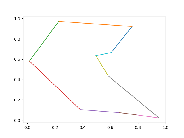
TSP Case Fully Connected

Now plot the optimal tour: \[ 1 \rightarrow 3 \rightarrow 8 \rightarrow 6 \rightarrow 10 \rightarrow 9 \rightarrow 5 \rightarrow 2 \rightarrow 4 \rightarrow 7 \rightarrow 1 \]

{linenos
1
2
3
4
5
6
7
8
tour_str = '1 3 8 6 10 9 5 2 4 7 1'
tour = list(map(lambda x: int(x), tour_str.split(' ')))

for i in range(0, len(tour)-1):
p1 = tour[i] - 1
p2 = tour[i + 1] - 1
plt.plot((x[p1],x[p2]),(y[p1],y[p2]))
plt.show()
TSP Case Minimal Tour

Python Code Illustrated

Init Graph Edges

Based on previous top down version, several changes are made. First, we need to have an edge between every 2 vertices and due to our matrix representation of the directed edge, edges of 2 directions are initialized.

{linenos
1
2
3
4
5
6
7
8
g: Graph = Graph(N)
for v in range(N):
for u in range(N):
diff_x = coordinates[v][0] - coordinates[u][0]
diff_y = coordinates[v][1] - coordinates[u][1]
dist: float = math.sqrt(diff_x * diff_x + diff_y * diff_y)
g.setDist(u, v, dist)
g.setDist(v, u, dist)

Auxilliary Variable to Track Tour Vertices

One major enhancement is to record the optimal tour during enumerating. We introduce another variable parent[bitstate][v] to track next vertex u, with shortest path.

{linenos
1
2
3
4
5
6
7
8
9
10
11
ret: float = FLOAT_INF
u_min: int = -1
for u in range(self.g.v_num):
if (state & (1 << u)) == 0:
s: float = self._recurse(u, state | 1 << u)
if s + edges[v][u] < ret:
ret = s + edges[v][u]
u_min = u
dp[state][v] = ret
self.parent[state][v] = u_min

After minimal tour distance is found, one optimal tour is formed with the help of parent variable.

{linenos
1
2
3
4
5
6
7
8
9
def _form_tour(self):
self.tour = [0]
bit = 0
v = 0
for _ in range(self.g.v_num - 1):
v = self.parent[bit][v]
self.tour.append(v)
bit = bit | (1 << v)
self.tour.append(0)

Note that for each test case, only one tour is given after "output". Our code may form a different tour but it has same distance as what the dataset generates, which can be verified by following code snippet. See full code on github.

{linenos
1
2
3
4
5
6
7
8
9
10
11
12
13
14
15
16
17
18
tsp: TSPSolver = TSPSolver(g)
tsp.solve()

output_dist: float = 0.0
output_tour = list(map(lambda x: int(x) - 1, output.split(' ')))
for v in range(1, len(output_tour)):
pre_v = output_tour[v-1]
curr_v = output_tour[v]
diff_x = coordinates[pre_v][0] - coordinates[curr_v][0]
diff_y = coordinates[pre_v][1] - coordinates[curr_v][1]
dist: float = math.sqrt(diff_x * diff_x + diff_y * diff_y)
output_dist += dist

passed = abs(tsp.dist - output_dist) < 10e-5
if passed:
print(f'passed dist={tsp.tour}')
else:
print(f'Min Tour Distance = {output_dist}, Computed Tour Distance = {tsp.dist}, Expected Tour = {output_tour}, Result = {tsp.tour}')

Travelling salesman problem (TSP) is a classic NP hard computer algorithmic problem. In this series, we will first solve TSP problem in an exact manner by ACing TSP on aizu with dynamic programming, and then move on to train a Pointer Network with Pytorch to obtain an approximate solution with deep learning and reinforcement learning technology. Complete episodes are listed as follows:

TSP Problem Review

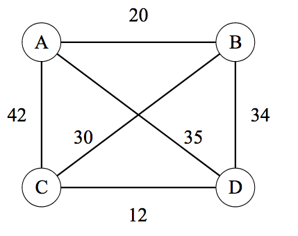
TSP can be modelled as a graph problem where both directed and undirected graphs and both completely or partially connected graphs are applicable. The following picture in Wikipedia TSP is an undirected but complete TSP with four vertices, A, B, C, D. TSP requries a tour with minimal total distance, starting from arbitrarily picked vertex and ending with the same node while covering all vertices exactly once. For example, \(A \rightarrow B \rightarrow C \rightarrow D \rightarrow A\) and \(A \rightarrow C \rightarrow B \rightarrow D \rightarrow A\) are valid tours and among all tours there is only one minimal distance value (though multiple tours with same minimum may exist).

Wikipedia 4 Vertices Example
Despite different types of graphs, notice that we can always employ an adjacency matrix to represent a graph. The above graph can thus be represented by this matrix

\[ \begin{matrix} & \begin{matrix}A&B&C&D\end{matrix} \\ \begin{matrix}A\\B\\C\\D\end{matrix} & \begin{bmatrix}-&20&42&35\\20&-&30&34\\42&30&-&12\\35&34&12&-\end{bmatrix}\\ \end{matrix} \]

Of course, typically, TSP problem takes the form of n cooridanates in a plane, corresponding to complete and undirected graph, because in plane every pair of vertices has one connected edge and the edge has same distance in both directions.

AIZU TSP Online Judge

AIZU has a TSP problem where a directed and incomplete graph with V vertices and E directed edges is given, and the output expects minimal total distance. For example below having 4 vertices and 6 edges.

This test case has minimal tour distance 16, with corresponding tour being \(0\rightarrow1\rightarrow3\rightarrow2\rightarrow0\), as shown in red edges. However, the AIZU problem may not have a valid result because not every pair of vertices is guaranteed to be connected. In that case, -1 is required, which can also be interpreted as infinity.

Brute Force Solution

A naive way is to enumerate all possible routes starting from vertex 0 and keep minimal total distance ever generated. Python code below illustrates a 4 point vertices graph.

{linenos
1
2
3
4
5
from itertools import permutations
v = [1,2,3]
p = permutations(v)
for t in list(p):
print([0] + list(t) + [0])

The possible routes are

{linenos
1
2
3
4
5
6
[0, 1, 2, 3, 0]
[0, 1, 3, 2, 0]
[0, 2, 1, 3, 0]
[0, 2, 3, 1, 0]
[0, 3, 1, 2, 0]
[0, 3, 2, 1, 0]
This approach has a runtime complexity of O(\(n!\)), which won't pass AIZU.

Dynamic Programming

To AC AIZU TSP, we need to have acceleration of the factorial runtime complexity by using bitmask dynamic programming. First, let us map visited state to a binary value. In the 4 vertices case, it's "0110" if node 2 and 1 already visited and ending at node 1. Besides, we need to track current vertex to start from. So we extend dp from one dimension to two dimensions \(dp[bitstate][v]\). In the example, it's \(dp["0110"][1]\). The transition formula is given by \[ dp[bitstate][v] = \min ( dp[bitstate \cup \{u\}][u] + dist(v,u) \mid u \notin bitstate ) \]

The resulting time complexity is O(\(n^2*2^n\) ), since there are \(2^n * n\) total states and for each state one more round loop is needed. Factorial and exponential functions are significantly different.

\(n!\) \(n^2*2^n\)
n=8 40320 16384
n=10 3628800 102400
n=12 479001600 589824
n=14 87178291200 3211264

Pause a second and think about why bitmask DP works here. Notice there are lots of redundant sub calls, one of which is hightlighted in red ellipse below.

In this episode, a straightforward top down memoization DP version is given in Python 3 and Java 8. Benefit of top down DP approach is that we don't need to consider topological ordering when permuting all states. Notice that there is a trick in Java, where each element of dp is initialized as Integer.MAX_VALUE, so that only one statement is needed to update new dp value.

1
res = Math.min(res, s + g.edges[v][u]);
However, the code simplicity is at cost of clarity and care should be taken when dealing with actual INF (not reachable case). In python version, we could have used the same trick, perhaps by intializing with a large long value representing INF. But for clarity, we manually handle different cases in if-else statements and mark intial value as -1 (INT_INF).

1
2
3
4
5
6
7
INT_INF = -1

if s != INT_INF and edges[v][u] != INT_INF:
if ret == INT_INF:
ret = s + edges[v][u]
else:
ret = min(ret, s + edges[v][u])

Below is complete AC code in Python 3 and Java 8. Also can be downloaded on github.

AIZU Java 8 Recursive Version

{linenos
1
2
3
4
5
6
7
8
9
10
11
12
13
14
15
16
17
18
19
20
21
22
23
24
25
26
27
28
29
30
31
32
33
34
35
36
37
38
39
40
41
42
43
44
45
46
47
48
49
50
51
52
53
54
55
56
57
58
59
60
61
62
63
64
65
66
67
68
69
70
71
72
73
74
75
76
77
78
79
80
81
82
// passed http://judge.u-aizu.ac.jp/onlinejudge/description.jsp?id=DPL_2_A
import java.util.Arrays;
import java.util.Scanner;

public class Main {
public static class Graph {
public final int V_NUM;
public final int[][] edges;

public Graph(int V_NUM) {
this.V_NUM = V_NUM;
this.edges = new int[V_NUM][V_NUM];
for (int i = 0; i < V_NUM; i++) {
Arrays.fill(this.edges[i], Integer.MAX_VALUE);
}
}

public void setDist(int src, int dest, int dist) {
this.edges[src][dest] = dist;
}

}

public static class TSP {
public final Graph g;
long[][] dp;

public TSP(Graph g) {
this.g = g;
}

public long solve() {
int N = g.V_NUM;
dp = new long[1 << N][N];
for (int i = 0; i < dp.length; i++) {
Arrays.fill(dp[i], -1);
}

long ret = recurse(0, 0);
return ret == Integer.MAX_VALUE ? -1 : ret;
}

private long recurse(int state, int v) {
int ALL = (1 << g.V_NUM) - 1;
if (dp[state][v] >= 0) {
return dp[state][v];
}
if (state == ALL && v == 0) {
dp[state][v] = 0;
return 0;
}
long res = Integer.MAX_VALUE;
for (int u = 0; u < g.V_NUM; u++) {
if ((state & (1 << u)) == 0) {
long s = recurse(state | 1 << u, u);
res = Math.min(res, s + g.edges[v][u]);
}
}
dp[state][v] = res;
return res;

}

}

public static void main(String[] args) {

Scanner in = new Scanner(System.in);
int V = in.nextInt();
int E = in.nextInt();
Graph g = new Graph(V);
while (E > 0) {
int src = in.nextInt();
int dest = in.nextInt();
int dist = in.nextInt();
g.setDist(src, dest, dist);
E--;
}
System.out.println(new TSP(g).solve());
}
}

AIZU Python 3 Recursive Version

{linenos
1
2
3
4
5
6
7
8
9
10
11
12
13
14
15
16
17
18
19
20
21
22
23
24
25
26
27
28
29
30
31
32
33
34
35
36
37
38
39
40
41
42
43
44
45
46
47
48
49
50
51
52
53
54
55
56
57
58
59
60
61
62
63
64
65
66
67
68
69
70
71
from typing import List

INT_INF = -1

class Graph:
v_num: int
edges: List[List[int]]

def __init__(self, v_num: int):
self.v_num = v_num
self.edges = [[INT_INF for c in range(v_num)] for r in range(v_num)]

def setDist(self, src: int, dest: int, dist: int):
self.edges[src][dest] = dist


class TSPSolver:
g: Graph
dp: List[List[int]]

def __init__(self, g: Graph):
self.g = g
self.dp = [[None for c in range(g.v_num)] for r in range(1 << g.v_num)]

def solve(self) -> int:
return self._recurse(0, 0)

def _recurse(self, v: int, state: int) -> int:
"""

:param v:
:param state:
:return: -1 means INF
"""
dp = self.dp
edges = self.g.edges

if dp[state][v] is not None:
return dp[state][v]

if (state == (1 << self.g.v_num) - 1) and (v == 0):
dp[state][v] = 0
return dp[state][v]

ret: int = INT_INF
for u in range(self.g.v_num):
if (state & (1 << u)) == 0:
s: int = self._recurse(u, state | 1 << u)
if s != INT_INF and edges[v][u] != INT_INF:
if ret == INT_INF:
ret = s + edges[v][u]
else:
ret = min(ret, s + edges[v][u])
dp[state][v] = ret
return ret


def main():
V, E = map(int, input().split())
g: Graph = Graph(V)
for _ in range(E):
src, dest, dist = map(int, input().split())
g.setDist(src, dest, dist)

tsp: TSPSolver = TSPSolver(g)
print(tsp.solve())


if __name__ == "__main__":
main()

Your browser is out-of-date!

Update your browser to view this website correctly. Update my browser now

×