This series, we deal with zero-sum turn-based board game algorithm, a sub type of combinatorial games. We start off with small search space problem, introduce classic algorithms and corresponding combinatorial gaming theory and ultimately end with modern approximating Deep RL techniques. From there, after stepping stone is laid, we are able to learn and appreciate how AlphaGo works. In this first episode, we illustrate 3 classic gaming problems in leetcode and solve them from brute force version to DP version then finally rewrite them using classic gaming algorithms, minimax and alpha beta pruning.

• Episode 1: Minimax and Alpha Beta Pruning in Leetcode

• Episode 2: Tic-Tac-Toe Problems in Leetcode and Solve the Game using Minimax

• Episode 3: Connect-N (Tic-Tac-Toe, Gomoku) OpenAI Gym GUI Environment

• Episode 4: Connect-N (Tic-Tac-Toe, Gomoku) AlphaGo Zero Self-Play MCTS Reinforcement Learning

Leetcode 292 Nim Game (Easy)

Let's start with an easy Leetcode gaming problem, Leetcode 292 Nim Game.

You are playing the following Nim Game with your friend: There is a heap of stones on the table, each time one of you take turns to remove 1 to 3 stones. The one who removes the last stone will be the winner. You will take the first turn to remove the stones.
Both of you are very clever and have optimal strategies for the game. Write a function to determine whether you can win the game given the number of stones in the heap.

Example:
Input: 4
Output: false
Explanation: If there are 4 stones in the heap, then you will never win the game;
No matter 1, 2, or 3 stones you remove, the last stone will always be removed by your friend.

Let \(f(n)\) be the result, either Win or Lose, when you take turn to make optimal move for the case of \(n\) stones. The first non trial case is \(f(4)\). By playing optimal strategies, it is equivalent to saying if there is any chance that leads to Win, you will definitely choose it. So you try 1, 2, 3 stones and see whether your opponent has any chance to win. Obviously, \(f(1) = f(2) = f(3) = Win\). Therefore, \(f(4)\) is guranteed to lose. Generally, the recurrence relation is given by \[ f(n) = \neg (f(n-1) \land f(n-2) \land f(n-3)) \]

1
2
3
4
5
6
7
8
9
10
11

# TLE
# Time Complexity: O(exponential)
class Solution_BruteForce:

    def canWinNim(self, n: int) -> bool:
        if n <= 3:
            return True
        for i in range(1, 4):
            if not self.canWinNim(n - i):
                return True
        return False

1
2
3
4
5
6
7
8
9
10
11
12

# RecursionError: maximum recursion depth exceeded in comparison n=1348820612
# Time Complexity: O(N)
class Solution_DP:
    from functools import lru_cache
    @lru_cache(maxsize=None)
    def canWinNim(self, n: int) -> bool:
        if n <= 3:
            return True
        for i in range(1, 4):
            if not self.canWinNim(n - i):
                return True
        return False

However, for this problem, lru_cache is not enough to AC because for large n, such as 1348820612, the implementation suffers from stack overflow. We can, of course, rewrite it in iterative forwarding loop manner. But still TLE.

1
2
3
4
5
6
7
8
9
10
11

# TLE for 1348820612
# Time Complexity: O(N)
class Solution:
    def canWinNim(self, n: int) -> bool:
        if n <= 3:
            return True
        last3, last2, last1 = True, True, True
        for i in range(4, n+1):
            this = not (last3 and last2 and last1)
            last3, last2, last1 = last2, last1, this
        return last1

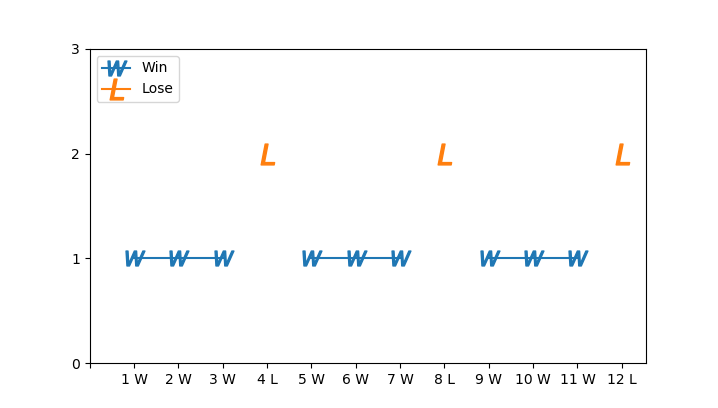
So AC code requires at most sublinear complexity. The last version also gives us some intuition that win lose may have period of 4. Actually, if you arrange all \(f(n)\) one by one, it's obvious that any \(n \mod 4 = 0\) leads to Lose and other cases lead to Win. Why? Suppose you start with \(4k+i (i=1,2,3)\), you can always remove \(i\) stones and leave \(4k\) stones to your opponent. Whatever he chooses, you are returned with situation \(4k_1 + i_1 (i_1 = 1,2,3)\). This pattern repeats until you have 1, 2, 3 remaining stones.

Below is one liner AC version.

1
2
3
4
5

# AC
# Time Complexity: O(1)
class Solution:
    def canWinNim(self, n: int) -> bool:
        return not (n % 4 == 0)

Leetcode 486 Predict the Winner (Medium)

Let's exercise a harder problem, Leetcode 486 Predict the Winner.

Given an array of scores that are non-negative integers. Player 1 picks one of the numbers from either end of the array followed by the player 2 and then player 1 and so on. Each time a player picks a number, that number will not be available for the next player. This continues until all the scores have been chosen. The player with the maximum score wins.
Given an array of scores, predict whether player 1 is the winner. You can assume each player plays to maximize his score.

Example 1:
Input: [1, 5, 2]
Output: False
Explanation: Initially, player 1 can choose between 1 and 2.
If he chooses 2 (or 1), then player 2 can choose from 1 (or 2) and 5. If player 2 chooses 5, then player 1 will be left with 1 (or 2).
So, final score of player 1 is 1 + 2 = 3, and player 2 is 5.
Hence, player 1 will never be the winner and you need to return False.

Example 2:
Input: [1, 5, 233, 7]
Output: True
Explanation: Player 1 first chooses 1. Then player 2 have to choose between 5 and 7. No matter which number player 2 choose, player 1 can choose 233.
Finally, player 1 has more score (234) than player 2 (12), so you need to return True representing player1 can win.

For a player, he can choose leftmost or rightmost one and leave remaining array to his opponent. Let us define maxDiff(l, r) to be the maximum difference current player can get, who is facing situation of subarray \([l, r]\).

\[ \begin{equation*} \operatorname{maxDiff}(l, r) = \max \begin{cases} nums[l] - \operatorname{maxDiff}(l + 1, r)\\\\ nums[r] - \operatorname{maxDiff}(l, r - 1) \end{cases} \end{equation*} \]

Runtime complexity can be written as following recurrence. \[ f(n) = 2f(n-1) = O(2^n) \]

Surprisingly, this time brute force version passed, but on the edge of rejection (6300ms).

1
2
3
4
5
6
7
8
9
10
11
12
13
14
15

# AC
# Time Complexity: O(2^N)
# Slow: 6300ms
from typing import List

class Solution:

    def maxDiff(self, l: int, r:int) -> int:
        if l == r:
            return self.nums[l]
        return max(self.nums[l] - self.maxDiff(l + 1, r), self.nums[r] - self.maxDiff(l, r - 1))

    def PredictTheWinner(self, nums: List[int]) -> bool:
        self.nums = nums
        return self.maxDiff(0, len(nums) - 1) >= 0

Again, be aware we have repeated computation over same node, for example, [1-2] node is expanded entirely for the second time when going from root to right node. Applying the same lru_cache trick, the one liner decorating maxDiff, we passed again with runtime complexity \(O(n^2)\) and running time 43ms, trial change but substantial improvement!

1
2
3
4
5
6
7
8
9
10
11
12
13
14
15
16
17

# AC
# Time Complexity: O(N^2)
# Fast: 43ms
from functools import lru_cache
from typing import List

class Solution:

    @lru_cache(maxsize=None)
    def maxDiff(self, l: int, r:int) -> int:
        if l == r:
            return self.nums[l]
        return max(self.nums[l] - self.maxDiff(l + 1, r), self.nums[r] - self.maxDiff(l, r - 1))

    def PredictTheWinner(self, nums: List[int]) -> bool:
        self.nums = nums
        return self.maxDiff(0, len(nums) - 1) >= 0

Leetcode 464 Can I Win (Medium)

A similar but slightly difficult problem is Leetcode 464 Can I Win, where bit mask with DP technique is employed.

In the "100 game," two players take turns adding, to a running total, any integer from 1..10. The player who first causes the running total to reach or exceed 100 wins.
What if we change the game so that players cannot re-use integers?
For example, two players might take turns drawing from a common pool of numbers of 1..15 without replacement until they reach a total >= 100.
Given an integer maxChoosableInteger and another integer desiredTotal, determine if the first player to move can force a win, assuming both players play optimally.
You can always assume that maxChoosableInteger will not be larger than 20 and desiredTotal will not be larger than 300.

Example
Input:
maxChoosableInteger = 10
desiredTotal = 11
Output:
false
Explanation:
No matter which integer the first player choose, the first player will lose.
The first player can choose an integer from 1 up to 10.
If the first player choose 1, the second player can only choose integers from 2 up to 10.
The second player will win by choosing 10 and get a total = 11, which is >= desiredTotal.
Same with other integers chosen by the first player, the second player will always win.

1
2
3
4
5
6
7
8
9
10
11
12
13
14
15
16
17
18
19
20
21
22
23
24

# AC
# Time Complexity: O:(2^m*m), m: maxChoosableInteger
class Solution:
    from functools import lru_cache
    @lru_cache(maxsize=None)
    def recurse(self, status: int, currentTotal: int) -> bool:
        for i in range(1, self.maxChoosableInteger + 1):
            if not (status >> i & 1):
                new_status = 1 << i | status
                if currentTotal + i >= self.desiredTotal:
                    return True
                if not self.recurse(new_status, currentTotal + i):
                    return True
        return False


    def canIWin(self, maxChoosableInteger: int, desiredTotal: int) -> bool:
        self.maxChoosableInteger = maxChoosableInteger
        self.desiredTotal = desiredTotal

        sum = maxChoosableInteger * (maxChoosableInteger + 1) / 2
        if sum < desiredTotal:
            return False
        return self.recurse(0, 0)

Because there are \(2^m\) states and for each state we need to probe at most \(m\) options, so the overall runtime complexity is \(O(m 2^m)\), where m is maxChoosableInteger.

Minimax Algorithm

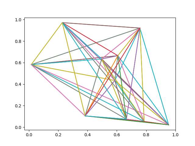
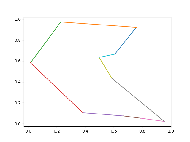
Up till now, we've seen serveral zero-sum turn based gaming in leetcode. In fact, there is more general algorithm for this type of gaming, named, minimax algorithm with alternate moves. The general setting is that, two players play in turn. The first player is trying to maximize game value and second player trying to minimize game value. For example, the following graph shows all nodes, labelled by its value. Computing from bottom up, the first player (max) can get optimal value -7, assuming both players play optimially.

Pseudo code in Python 3 is listed below.

1
2
3
4
5
6
7
8
9
10
11
12
13

def minimax(node: Node, depth: int, maximizingPlayer: bool) -> int:
    if depth == 0 or is_terminal(node):
        return evaluate_terminal(node)
    if maximizingPlayer:
        value:int = −∞
        for child in node:
            value = max(value, minimax(child, depth − 1, False))
        return value
    else: # minimizing player
        value := +∞
        for child in node:
            value = min(value, minimax(child, depth − 1, True))
        return value

Minimax: 486 Predict the Winner

We know leetcode 486 Predict the Winner is zero-sum turn-based game. Hence, theoretically, we can come up with a minimax algorithm for it. But the difficulty lies in how we define value or utility for it. In previous section, we've defined maxDiff(l, r) to be the maximum difference for current player, who is left with sub array \([l, r]\). In the most basic case, where only one element x is left, it's intuitive to define +x for max player and -x for min player. If we merge it with minimax algorithm, it's naturally follows that, the total reward got by max player is \(+a_1 + a_2 + ... = A\) and reward by min player is \(-b_1 - b_2 - ... = -B\), and max player aims to \(max(A-B)\) while min player aims to \(min(A-B)\). With that in mind, code is not hard to implement.

1
2
3
4
5
6
7
8
9
10
11
12
13
14
15
16
17
18
19
20
21
22
23
24
25

# AC
from functools import lru_cache
from typing import List

class Solution:
    # max_player: max(A - B)
    # min_player: min(A - B)
    @lru_cache(maxsize=None)
    def minimax(self, l: int, r: int, isMaxPlayer: bool) -> int:
        if l == r:
            return self.nums[l] * (1 if isMaxPlayer else -1)

        if isMaxPlayer:
            return max(
                self.nums[l] + self.minimax(l + 1, r, not isMaxPlayer),
                self.nums[r] + self.minimax(l, r - 1, not isMaxPlayer))
        else:
            return min(
                -self.nums[l] + self.minimax(l + 1, r, not isMaxPlayer),
                -self.nums[r] + self.minimax(l, r - 1, not isMaxPlayer))

    def PredictTheWinner(self, nums: List[int]) -> bool:
        self.nums = nums
        v = self.minimax(0, len(nums) - 1, True)
        return v >= 0

Minimax: 464 Can I Win

For this problem, as often processed in other win-lose-tie game without intermediate intrinsic value, it's typically to define +1 in case max player wins, -1 for min player and 0 for tie. Note the shortcut case for both player. For example, the max player can report Win (value=1) once he finds winning condition (>=desiredTotal) is satisfied during enumerating possible moves he can make. This also makes sense since if he gets 1 during maxing, there can not be other value for further probing that is finally returned. The same optimization will be generalized in the next improved algorithm, alpha beta pruning.

1
2
3
4
5
6
7
8
9
10
11
12
13
14
15
16
17
18
19
20
21
22
23
24
25
26
27
28
29
30
31
32

# AC
class Solution:
    from functools import lru_cache
    @lru_cache(maxsize=None)
    # currentTotal < desiredTotal
    def minimax(self, status: int, currentTotal: int, isMaxPlayer: bool) -> int:
        import math
        if status == self.allUsed:
            return 0  # draw: no winner

        if isMaxPlayer:
            value = -math.inf
            for i in range(1, self.maxChoosableInteger + 1):
                if not (status >> i & 1):
                    new_status = 1 << i | status
                    if currentTotal + i >= self.desiredTotal:
                        return 1  # shortcut
                    value = max(value, self.minimax(new_status, currentTotal + i, not isMaxPlayer))
                    if value == 1:
                        return 1
            return value
        else:
            value = math.inf
            for i in range(1, self.maxChoosableInteger + 1):
                if not (status >> i & 1):
                    new_status = 1 << i | status
                    if currentTotal + i >= self.desiredTotal:
                        return -1  # shortcut
                    value = min(value, self.minimax(new_status, currentTotal + i, not isMaxPlayer))
                    if value == -1:
                        return -1
            return value

Alpha-Beta Pruning

We sensed there is space of optimaization during searching, as illustrated in 464 Can I Win minimax algorithm. Let's formalize this idea, called alpha beta pruning. For each node, we maintain two values alpha and beta, which represent the minimum score that the maximizing player is assured of and the maximum score that the minimizing player is assured of, respectively. The root node has initial alpha = −∞ and beta = +∞, forming valid duration [−∞, +∞]. During top down traversal, child node inherits alpha beta value from its parent node, for example, [alpha, beta], if the updated alpha or beta in the child node no longer forms a valid interval, the branch can be pruned and return immediately. Take following example in Wikimedia for example.

1. Root node, intially: alpha = −∞, beta = +∞

2. Root node, after 4 is returned, alpha = 4, beta = +∞

3. Root node, after 5 is returned, alpha = 5, beta = +∞

4. Rightmost Min node, intially: alpha = 5, beta = +∞

5. Rightmost Min node, after 1 is returned: alpha = 5, beta = 1

Here we see [5, 1] no longer is valid interval, so it returns without further probing his 2nd and 3rd child. Why? because if the other child returns value > 1, say 2, it will be replaced by 1 as it's a min node with guarenteed value 1. If the other child returns value < 1, it will be abandoned by root node, a max node, which has already guarenteed to have value >=5. So in this situation, whatever other children return does not impact anything.

Pseudo code in Python 3 is listed below.

1
2
3
4
5
6
7
8
9
10
11
12
13
14
15
16
17
18
19

def alpha_beta(node: Node, depth: int, α: int, β: int, maximizingPlayer: bool) -> int:
    if depth == 0 or is_terminal(node):
        return evaluate_terminal(node)
    if maximizingPlayer:
        value: int = −∞
        for child in node:
            value = max(value, alphabeta(child, depth − 1, α, β, False))
            α = max(α, value)
            if α >= β:
                break # β cut-off
        return value
    else:
        value: int = +∞
        for child in node:
            value = min(value, alphabeta(child, depth − 1, α, β, True))
            β = min(β, value)
            if β <= α:
                break # α cut-off
        return value

Alpha-Beta Pruning: 486 Predict the Winner

1
2
3
4
5
6
7
8
9
10
11
12
13
14
15
16
17
18
19
20
21
22
23
24
25
26
27
28
29

# AC
import math
from functools import lru_cache
from typing import List

class Solution:
    def alpha_beta(self, l: int, r: int, curr: int, isMaxPlayer: bool, alpha: int, beta: int) -> int:
        if l == r:
            return curr + self.nums[l] * (1 if isMaxPlayer else -1)

        if isMaxPlayer:
            ret = self.alpha_beta(l + 1, r, curr + self.nums[l], not isMaxPlayer, alpha, beta)
            alpha = max(alpha, ret)
            if alpha >= beta:
                return alpha
            ret = max(ret, self.alpha_beta(l, r - 1, curr + self.nums[r], not isMaxPlayer, alpha, beta))
            return ret
        else:
            ret = self.alpha_beta(l + 1, r, curr - self.nums[l], not isMaxPlayer, alpha, beta)
            beta = min(beta, ret)
            if alpha >= beta:
                return beta
            ret = min(ret, self.alpha_beta(l, r - 1, curr - self.nums[r], not isMaxPlayer, alpha, beta))
            return ret

    def PredictTheWinner(self, nums: List[int]) -> bool:
        self.nums = nums
        v = self.alpha_beta(0, len(nums) - 1, 0, True, -math.inf, math.inf)
        return v >= 0

Alpha-Beta Pruning: 464 Can I Win

1
2
3
4
5
6
7
8
9
10
11
12
13
14
15
16
17
18
19
20
21
22
23
24
25
26
27
28
29
30
31
32
33
34

# AC
class Solution:
    from functools import lru_cache
    @lru_cache(maxsize=None)
    # currentTotal < desiredTotal
    def alpha_beta(self, status: int, currentTotal: int, isMaxPlayer: bool, alpha: int, beta: int) -> int:
        import math
        if status == self.allUsed:
            return 0  # draw: no winner

        if isMaxPlayer:
            value = -math.inf
            for i in range(1, self.maxChoosableInteger + 1):
                if not (status >> i & 1):
                    new_status = 1 << i | status
                    if currentTotal + i >= self.desiredTotal:
                        return 1  # shortcut
                    value = max(value, self.alpha_beta(new_status, currentTotal + i, not isMaxPlayer, alpha, beta))
                    alpha = max(alpha, value)
                    if alpha >= beta:
                        return value
            return value
        else:
            value = math.inf
            for i in range(1, self.maxChoosableInteger + 1):
                if not (status >> i & 1):
                    new_status = 1 << i | status
                    if currentTotal + i >= self.desiredTotal:
                        return -1  # shortcut
                    value = min(value, self.alpha_beta(new_status, currentTotal + i, not isMaxPlayer, alpha, beta))
                    beta = min(beta, value)
                    if alpha >= beta:
                        return value
            return value

C++, Java, Javascript for 486 Predict the Winner

As a bonus, we AC leetcode 486 in C++, Java and Javascript with a bottom up iterative DP. We illustrate this method for other languages not just because lru_cache is available in non Python languages, but also because there are other ways to solve the problem. Notice the topological ordering of DP dependency, building larger DP based on smaller and solved ones. In addition, it's worth mentioning that this approach is guaranteed to have \(n^2\) loops but top down caching approach can have sub \(n^2\) loops.

Java AC Code

1
2
3
4
5
6
7
8
9
10
11
12
13
14
15
16
17
18
19

// AC
class Solution {
    public boolean PredictTheWinner(int[] nums) {
        int n = nums.length;
        int[][] dp = new int[n][n];
        for (int i = 0; i < n; i++) {
            dp[i][i] = nums[i];
        }

        for (int l = n - 1; l >= 0; l--) {
            for (int r = l + 1; r < n; r++) {
                dp[l][r] = Math.max(
                        nums[l] - dp[l + 1][r],
                        nums[r] - dp[l][r - 1]);
            }
        }
        return dp[0][n - 1] >= 0;
    }
}

C++ AC Code

1
2
3
4
5
6
7
8
9
10
11
12
13
14
15
16
17

// AC
class Solution {
public:
    bool PredictTheWinner(vector<int>& nums) {
        int n = nums.size();
        vector<vector<int>> dp(n, vector<int>(n, 0));
        for (int i = 0; i < n; i++) {
          dp[i][i] = nums[i];
        }
        for (int l = n - 1; l >= 0; l--) {
            for (int r = l + 1; r < n; r++) {
                dp[l][r] = max(nums[l] - dp[l + 1][r], nums[r] - dp[l][r - 1]);
            }
        }
        return dp[0][n - 1] >= 0;
    }
};

Javascript AC Code

1
2
3
4
5
6
7
8
9
10
11
12
13
14
15
16
17
18
19
20

/**
 * @param {number[]} nums
 * @return {boolean}
 */
var PredictTheWinner = function(nums) {
    const n = nums.length;
    const dp = new Array(n).fill().map(() => new Array(n));

    for (let i = 0; i < n; i++) {
      dp[i][i] = nums[i];
    }
  
    for (let l = n - 1; l >=0; l--) {
        for (let r = i + 1; r < n; r++) {
            dp[l][r] = Math.max(nums[l] - dp[l + 1][r],nums[r] - dp[l][r - 1]);
        }
    }
  
    return dp[0][n-1] >=0;
};

This is second episode of series: TSP From DP to Deep Learning.

• Episode 1: AC TSP on AIZU with recursive DP
• Episode 2: TSP DP on a Euclidean Dataset
• Episode 3: Pointer Networks in PyTorch
• Episode 4: Search for Most Likely Sequence
• Episode 5: Reinforcement Learning PyTorch Implementation

AIZU TSP Bottom Up Iterative DP

In last episode, we provided a top down recursive DP in Python 3 and Java 8. Now we continue to improve and convert it to bottom up iterative DP version. Below is a graph with 3 vertices, the top down recursive calls are completely drawn.

Looking from bottom up, we could identify corresponding topological computing order with ease. First, we compute all bit states with 3 ones, then 2 ones, then 1 one.

Pseudo Java code below.

1
2
3
4
5
6
7
8
9
10
11
12
13
14
15
16

for (int bitset_num = N; bitset_num >=0; bitset_num++) {
	while(hasNextCombination(bitset_num)) {
		int state = nextCombination(bitset_num);
		// compute dp[state][v], v-th bit is set in state
		for (int v = 0; v < n; v++) {
			for (int u = 0; u < n; u++) {
				// for each u not reached by this state
				if (!include(state, u)) {
					dp[state][v] = min(dp[state][v], 
						dp[new_state_include_u][u] + dist[v][u]);
				}
			}
		}
	}
}

For example, dp[00010][1] is the min distance starting from vertex 0, and just arriving at vertex 1: \(0 \rightarrow 1 \rightarrow ? \rightarrow ? \rightarrow ? \rightarrow 0\). In order to find out total min distance, we need to enumerate all possible u for first question mark. \[ (0 \rightarrow 1) + \begin{align*} \min \left\lbrace \begin{array}{r@{}l} 2 \rightarrow ? \rightarrow ? \rightarrow 0 + dist(1,2) \qquad\text{ new_state=[00110][2] } \qquad\\\\ 3 \rightarrow ? \rightarrow ? \rightarrow 0 + dist(1,3) \qquad\text{ new_state=[01010][3] } \qquad\\\\ 4 \rightarrow ? \rightarrow ? \rightarrow 0 + dist(1,4) \qquad\text{ new_state=[10010][4] } \qquad \end{array} \right. \end{align*} \]

Java Iterative DP Code

AC code in Python 3 and Java 8. Illustrate core Java code below.

1
2
3
4
5
6
7
8
9
10
11
12
13
14
15
16
17
18
19
20

public long solve() {
	int N = g.V_NUM;
	long[][] dp = new long[1 << N][N];
	// init dp[][] with MAX
	for (int i = 0; i < dp.length; i++) {
		Arrays.fill(dp[i], Integer.MAX_VALUE);
	}
	dp[(1 << N) - 1][0] = 0;

	for (int state = (1 << N) - 2; state >= 0; state--) {
		for (int v = 0; v < N; v++) {
			for (int u = 0; u < N; u++) {
				if (((state >> u) & 1) == 0) {
					dp[state][v] = Math.min(dp[state][v], dp[state | 1 << u][u] + g.edges[v][u]);
				}
			}
		}
	}
	return dp[0][0] == Integer.MAX_VALUE ? -1 : dp[0][0];
}

In this way, runtime complexity can be spotted easily, three for loops leading to O(\(2^n * n * n\)) = O(\(2^n*n^2\) ).

DP on Euclidean Dataset

So far, TSP DP has been crystal clear and we move forward to introducing PTR_NET dataset on Google Drive by Oriol Vinyals who is the author of Pointer Networks. Each line in the dataset has the following pattern:

1

x0, y0, x1, y1, ... output 1 v1 v2 v3 ... 1

It first lists n points in (x, y) coordinate, followed by "output", then followed by one of the minimal distance tours, starting and ending with vertex 1 (indexed from 1 not 0).

Some examples of 10 vertices are:

1
2
3
4

0.607122 0.664447 0.953593 0.021519 0.757626 0.921024 0.586376 0.433565 0.786837 0.052959 0.016088 0.581436 0.496714 0.633571 0.227777 0.971433 0.665490 0.074331 0.383556 0.104392 output 1 3 8 6 10 9 5 2 4 7 1 
0.930534 0.747036 0.277412 0.938252 0.794592 0.794285 0.961946 0.261223 0.070796 0.384302 0.097035 0.796306 0.452332 0.412415 0.341413 0.566108 0.247172 0.890329 0.429978 0.232970 output 1 3 2 9 6 5 8 7 10 4 1 
0.686712 0.087942 0.443054 0.277818 0.494769 0.985289 0.559706 0.861138 0.532884 0.351913 0.712561 0.199273 0.554681 0.657214 0.909986 0.277141 0.931064 0.639287 0.398927 0.406909 output 1 5 2 10 7 4 3 9 8 6 1 

Plot first example using code below.

1
2
3
4
5
6
7
8
9
10
11
12
13
14
15
16
17
18

import matplotlib.pyplot as plt
points='0.607122 0.664447 0.953593 0.021519 0.757626 0.921024 0.586376 0.433565 0.786837 0.052959 0.016088 0.581436 0.496714 0.633571 0.227777 0.971433 0.665490 0.074331 0.383556 0.104392'
float_list = list(map(lambda x: float(x), points.split(' ')))

x,y = [],[]
for idx, p in enumerate(float_list):
  if idx % 2 == 0:
    x.append(p)
  else:
    y.append(p)

for i in range(0, len(x)):
  for j in range(0, len(x)):
    if i == j:
      continue
    plt.plot((x[i],x[j]),(y[i],y[j]))

plt.show()

Now plot the optimal tour: \[ 1 \rightarrow 3 \rightarrow 8 \rightarrow 6 \rightarrow 10 \rightarrow 9 \rightarrow 5 \rightarrow 2 \rightarrow 4 \rightarrow 7 \rightarrow 1 \]

1
2
3
4
5
6
7
8

tour_str = '1 3 8 6 10 9 5 2 4 7 1'
tour = list(map(lambda x: int(x), tour_str.split(' ')))

for i in range(0, len(tour)-1):
  p1 = tour[i] - 1
  p2 = tour[i + 1] - 1
  plt.plot((x[p1],x[p2]),(y[p1],y[p2]))
plt.show()

Python Code Illustrated

Init Graph Edges

Based on previous top down version, several changes are made. First, we need to have an edge between every 2 vertices and due to our matrix representation of the directed edge, edges of 2 directions are initialized.

1
2
3
4
5
6
7
8

g: Graph = Graph(N)
for v in range(N):
	for u in range(N):
		diff_x = coordinates[v][0] - coordinates[u][0]
		diff_y = coordinates[v][1] - coordinates[u][1]
		dist: float = math.sqrt(diff_x * diff_x + diff_y * diff_y)
		g.setDist(u, v, dist)
		g.setDist(v, u, dist)

Auxilliary Variable to Track Tour Vertices

One major enhancement is to record the optimal tour during enumerating. We introduce another variable parent[bitstate][v] to track next vertex u, with shortest path.

1
2
3
4
5
6
7
8
9
10
11

ret: float = FLOAT_INF
u_min: int = -1
	for u in range(self.g.v_num):
		if (state & (1 << u)) == 0:
			s: float = self._recurse(u, state | 1 << u)
				if s + edges[v][u] < ret:
					ret = s + edges[v][u]
					u_min = u
	dp[state][v] = ret
	self.parent[state][v] = u_min

After minimal tour distance is found, one optimal tour is formed with the help of parent variable.

1
2
3
4
5
6
7
8
9

def _form_tour(self):
	self.tour = [0]
	bit = 0
	v = 0
	for _ in range(self.g.v_num - 1):
		v = self.parent[bit][v]
		self.tour.append(v)
		bit = bit | (1 << v)
	self.tour.append(0)

Note that for each test case, only one tour is given after "output". Our code may form a different tour but it has same distance as what the dataset generates, which can be verified by following code snippet. See full code on github.

1
2
3
4
5
6
7
8
9
10
11
12
13
14
15
16
17
18

tsp: TSPSolver = TSPSolver(g)
tsp.solve()

output_dist: float = 0.0
output_tour = list(map(lambda x: int(x) - 1, output.split(' ')))
for v in range(1, len(output_tour)):
	pre_v = output_tour[v-1]
	curr_v = output_tour[v]
	diff_x = coordinates[pre_v][0] - coordinates[curr_v][0]
	diff_y = coordinates[pre_v][1] - coordinates[curr_v][1]
	dist: float = math.sqrt(diff_x * diff_x + diff_y * diff_y)
	output_dist += dist

	passed = abs(tsp.dist - output_dist) < 10e-5
	if passed:
		print(f'passed dist={tsp.tour}')
	else:
		print(f'Min Tour Distance = {output_dist}, Computed Tour Distance = {tsp.dist}, Expected Tour = {output_tour}, Result = {tsp.tour}')

Travelling salesman problem (TSP) is a classic NP hard computer algorithmic problem. In this series, we will first solve TSP problem in an exact manner by ACing TSP on aizu with dynamic programming, and then move on to train a Pointer Network with Pytorch to obtain an approximate solution with deep learning and reinforcement learning technology. Complete episodes are listed as follows:

• Episode 1: AC TSP on AIZU with recursive DP

• Episode 2: TSP DP on a Euclidean Dataset

• Episode 3: Pointer Networks in PyTorch

• Episode 4: Search for Most Likely Sequence

• Episode 5: Reinforcement Learning PyTorch Implementation

TSP Problem Review

TSP can be modelled as a graph problem where both directed and undirected graphs and both completely or partially connected graphs are applicable. The following picture in Wikipedia TSP is an undirected but complete TSP with four vertices, A, B, C, D. TSP requries a tour with minimal total distance, starting from arbitrarily picked vertex and ending with the same node while covering all vertices exactly once. For example, \(A \rightarrow B \rightarrow C \rightarrow D \rightarrow A\) and \(A \rightarrow C \rightarrow B \rightarrow D \rightarrow A\) are valid tours and among all tours there is only one minimal distance value (though multiple tours with same minimum may exist).

Of course, typically, TSP problem takes the form of n cooridanates in a plane, corresponding to complete and undirected graph, because in plane every pair of vertices has one connected edge and the edge has same distance in both directions.

AIZU TSP Online Judge

AIZU has a TSP problem where a directed and incomplete graph with V vertices and E directed edges is given, and the output expects minimal total distance. For example below having 4 vertices and 6 edges.

This test case has minimal tour distance 16, with corresponding tour being \(0\rightarrow1\rightarrow3\rightarrow2\rightarrow0\), as shown in red edges. However, the AIZU problem may not have a valid result because not every pair of vertices is guaranteed to be connected. In that case, -1 is required, which can also be interpreted as infinity.

Brute Force Solution

A naive way is to enumerate all possible routes starting from vertex 0 and keep minimal total distance ever generated. Python code below illustrates a 4 point vertices graph.

1
2
3
4
5

from itertools import permutations
v = [1,2,3]
p = permutations(v)
for t in list(p):
  print([0] + list(t) + [0])

The possible routes are

1
2
3
4
5
6

[0, 1, 2, 3, 0]
[0, 1, 3, 2, 0]
[0, 2, 1, 3, 0]
[0, 2, 3, 1, 0]
[0, 3, 1, 2, 0]
[0, 3, 2, 1, 0]

Dynamic Programming

To AC AIZU TSP, we need to have acceleration of the factorial runtime complexity by using bitmask dynamic programming. First, let us map visited state to a binary value. In the 4 vertices case, it's "0110" if node 2 and 1 already visited and ending at node 1. Besides, we need to track current vertex to start from. So we extend dp from one dimension to two dimensions \(dp[bitstate][v]\). In the example, it's \(dp["0110"][1]\). The transition formula is given by \[ dp[bitstate][v] = \min ( dp[bitstate \cup \{u\}][u] + dist(v,u) \mid u \notin bitstate ) \]

The resulting time complexity is O(\(n^2*2^n\) ), since there are \(2^n * n\) total states and for each state one more round loop is needed. Factorial and exponential functions are significantly different.

Pause a second and think about why bitmask DP works here. Notice there are lots of redundant sub calls, one of which is hightlighted in red ellipse below.

In this episode, a straightforward top down memoization DP version is given in Python 3 and Java 8. Benefit of top down DP approach is that we don't need to consider topological ordering when permuting all states. Notice that there is a trick in Java, where each element of dp is initialized as Integer.MAX_VALUE, so that only one statement is needed to update new dp value.

1

res = Math.min(res, s + g.edges[v][u]);

1
2
3
4
5
6
7

INT_INF = -1

if s != INT_INF and edges[v][u] != INT_INF:
    if ret == INT_INF:
        ret = s + edges[v][u]
    else:
        ret = min(ret, s + edges[v][u])

Below is complete AC code in Python 3 and Java 8. Also can be downloaded on github.

AIZU Java 8 Recursive Version

1
2
3
4
5
6
7
8
9
10
11
12
13
14
15
16
17
18
19
20
21
22
23
24
25
26
27
28
29
30
31
32
33
34
35
36
37
38
39
40
41
42
43
44
45
46
47
48
49
50
51
52
53
54
55
56
57
58
59
60
61
62
63
64
65
66
67
68
69
70
71
72
73
74
75
76
77
78
79
80
81
82

// passed http://judge.u-aizu.ac.jp/onlinejudge/description.jsp?id=DPL_2_A
import java.util.Arrays;
import java.util.Scanner;

public class Main {
    public static class Graph {
        public final int V_NUM;
        public final int[][] edges;

        public Graph(int V_NUM) {
            this.V_NUM = V_NUM;
            this.edges = new int[V_NUM][V_NUM];
            for (int i = 0; i < V_NUM; i++) {
                Arrays.fill(this.edges[i], Integer.MAX_VALUE);
            }
        }
    
        public void setDist(int src, int dest, int dist) {
            this.edges[src][dest] = dist;
        }
    
    }
    
    public static class TSP {
        public final Graph g;
        long[][] dp;
    
        public TSP(Graph g) {
            this.g = g;
        }
    
        public long solve() {
            int N = g.V_NUM;
            dp = new long[1 << N][N];
            for (int i = 0; i < dp.length; i++) {
                Arrays.fill(dp[i], -1);
            }
    
            long ret = recurse(0, 0);
            return ret == Integer.MAX_VALUE ? -1 : ret;
        }
    
        private long recurse(int state, int v) {
            int ALL = (1 << g.V_NUM) - 1;
            if (dp[state][v] >= 0) {
                return dp[state][v];
            }
            if (state == ALL && v == 0) {
                dp[state][v] = 0;
                return 0;
            }
            long res = Integer.MAX_VALUE;
            for (int u = 0; u < g.V_NUM; u++) {
                if ((state & (1 << u)) == 0) {
                    long s = recurse(state | 1 << u, u);
                    res = Math.min(res, s + g.edges[v][u]);
                }
            }
            dp[state][v] = res;
            return res;
    
        }
    
    }
    
    public static void main(String[] args) {
    
        Scanner in = new Scanner(System.in);
        int V = in.nextInt();
        int E = in.nextInt();
        Graph g = new Graph(V);
        while (E > 0) {
            int src = in.nextInt();
            int dest = in.nextInt();
            int dist = in.nextInt();
            g.setDist(src, dest, dist);
            E--;
        }
        System.out.println(new TSP(g).solve());
    }
}

AIZU Python 3 Recursive Version

1
2
3
4
5
6
7
8
9
10
11
12
13
14
15
16
17
18
19
20
21
22
23
24
25
26
27
28
29
30
31
32
33
34
35
36
37
38
39
40
41
42
43
44
45
46
47
48
49
50
51
52
53
54
55
56
57
58
59
60
61
62
63
64
65
66
67
68
69
70
71

from typing import List

INT_INF = -1

class Graph:
    v_num: int
    edges: List[List[int]]

    def __init__(self, v_num: int):
        self.v_num = v_num
        self.edges = [[INT_INF for c in range(v_num)] for r in range(v_num)]
    
    def setDist(self, src: int, dest: int, dist: int):
        self.edges[src][dest] = dist


class TSPSolver:
    g: Graph
    dp: List[List[int]]

    def __init__(self, g: Graph):
        self.g = g
        self.dp = [[None for c in range(g.v_num)] for r in range(1 << g.v_num)]
    
    def solve(self) -> int:
        return self._recurse(0, 0)
    
    def _recurse(self, v: int, state: int) -> int:
        """
    
        :param v:
        :param state:
        :return: -1 means INF
        """
        dp = self.dp
        edges = self.g.edges
    
        if dp[state][v] is not None:
            return dp[state][v]
    
        if (state == (1 << self.g.v_num) - 1) and (v == 0):
            dp[state][v] = 0
            return dp[state][v]
    
        ret: int = INT_INF
        for u in range(self.g.v_num):
            if (state & (1 << u)) == 0:
                s: int = self._recurse(u, state | 1 << u)
                if s != INT_INF and edges[v][u] != INT_INF:
                    if ret == INT_INF:
                        ret = s + edges[v][u]
                    else:
                        ret = min(ret, s + edges[v][u])
        dp[state][v] = ret
        return ret


def main():
    V, E = map(int, input().split())
    g: Graph = Graph(V)
    for _ in range(E):
        src, dest, dist = map(int, input().split())
        g.setDist(src, dest, dist)

    tsp: TSPSolver = TSPSolver(g)
    print(tsp.solve())


if __name__ == "__main__":
    main()