#PyTorch

This is fifth episode of series: TSP From DP to Deep Learning. In this episode, we turn to Reinforcement Learning technology, in particular, a model-free policy gradient method that embeds pointer network to learn minimal tour without supervised best tour label in dataset. Full list of this series is listed below.

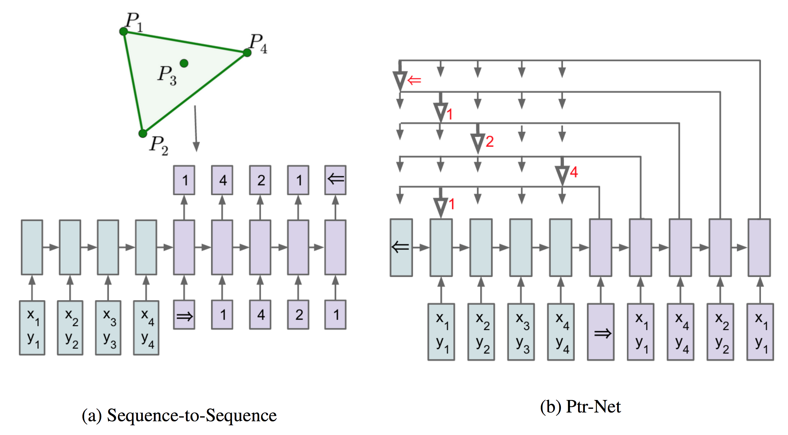
Pointer Network Refresher

In previous episode Pointer Networks in PyTorch, we implemented Pointer Networks in PyTorch with a 2D Euclidean dataset.

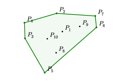
Recall that the input is a graph as a sequence of \(n\) cities in a two dimensional space

\[ s=\{\mathbf{x_i}\}_{i=1}^n, \mathbf{x}_{i} \in \mathbb{R}^{2} \]

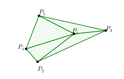
The output is a permutation of the points \(\pi\), that visits each city exactly once and returns to starting point with minimal distance.

Let us define the total distance of a \(\pi\) with respect to \(s\) as \(L\)

\[ L(\pi | s)=\left\|\mathbf{x}_{\pi(n)}-\mathbf{x}_{\pi(1)}\right\|_{2}+\sum_{i=1}^{n-1}\left\|\mathbf{x}_{\pi(i)}-\mathbf{x}_{\pi(i+1)}\right\|_{2} \]

The stochastic policy \(p(\pi | s; \theta)\), parameterized by \(\theta\), is aiming to assign high probabilities to short tours and low probabilities to long tours. The joint probability assumes independency to allow factorization.

\[ p(\pi | s; \theta) = \prod_{i=1}^{n} p\left({\pi(i)} | {\pi(1)}, \ldots, {\pi(i-1)} , s; \theta\right) \]

The loss of the model is cross entropy between the network’s output probabilities \(\pi\) and the best tour \(\hat{\pi}\) generated by a TSP solver.

Contribution made by Pointer networks is that it addressed the constraint in that it allows for dynamic index value given by the particular test case, instead of from a fixed-size vocabulary.

Reinforcement Learning

Neural Combinatorial Optimization with Reinforcement Learning combines the power of Reinforcement Learning (RL) and Deep Learning to further eliminate the constraint required by Pointer Networks that the training dataset has to have supervised labels of best tour. With deep RL, test cases do not need to have a solution which is common pattern in deep RL. In the paper, a model-free policy-based RL method is adopted.

Model-Free Policy Gradient Methods

In the authoritative RL book, chapter 8 Planning and Learning with Tabular Methods, there are two major approaches in RL. One is model-based RL and the other is model-free RL. Distinction between the two relies on concept of model, which is stated as follows:

By a model of the environment we mean anything that an agent can use to predict how the environment will respond to its actions.

So model-based methods demand a model of the environment, and hence dynamic programming and heuristic search fall into this category. With model in mind, utility of the state can be computed in various ways and planning stage that essentially builds policy is needed before agent can take any action. In contrast, model-free methods, without building a model, are more direct, ignoring irrelevant information and just focusing on the policy which is ultimately needed. Typical examples of model-free methods are Monte Carlo Control and Temporal-Difference Learning. >Model-based methods rely on planning as their primary component, while model-free methods primarily rely on learning.

In TSP problem, the model is fully determined by all points given, and no feedback is generated for each decision made. So it's unclear to how to map state value with a tour. Therefore, we turn to model-free methods. In chapter 13 Policy Gradient Methods, a particular approximation model-free method that learns a parameterized policy that can select actions without consulting a value function. This approach fits perfectly with aforementioned pointer networks where the parameterized policy \(p(\pi | s; \theta)\) is already defined.

Training objective is obvious, the expected tour length of \(\pi_\theta\) which, given an input graph \(s\)

\[ J(\theta | s) = \mathbb{E}_{\pi \sim p_{\theta}(\cdot | s)} L(\pi | s) \]

Monte Carlo Policy Gradient: REINFORCE with Baseline

In order to find largest reward, a typical way is to optimize the parameters \(\theta\) in the direction of derivative: \(\nabla_{\theta} J(\theta | s)\).

\[ \nabla_{\theta} J(\theta | s)=\nabla_{\theta} \mathbb{E}_{\pi \sim p_{\theta}(\cdot | s)} L(\pi | s) \]

RHS of equation above is the derivative of expectation that we have no idea how to compute or approximate. Here comes the well-known REINFORCE trick that turns it into form of expectation of derivative, which can be approximated easily with Monte Carlo sampling, where the expectation is replaced by averaging.

\[ \nabla_{\theta} J(\theta | s)=\mathbb{E}_{\pi \sim p_{\theta}(. | s)}\left[L(\pi | s) \nabla_{\theta} \log p_{\theta}(\pi | s)\right] \]

Another common trick, subtracting a baseline \(b(s)\), leads the derivative of reward to the following equation. Note that \(b(s)\) denotes a baseline function that must not depend on \(\pi\). \[ \nabla_{\theta} J(\theta | s)=\mathbb{E}_{\pi \sim p_{\theta}(. | s)}\left[(L(\pi | s)-b(s)) \nabla_{\theta} \log p_{\theta}(\pi | s)\right] \]

The trick is explained in as:

Because the baseline could be uniformly zero, this update is a strict generalization of REINFORCE. In general, the baseline leaves the expected value of the update unchanged, but it can have a large effect on its variance.

Finally, the equation can be approximated with Monte Carlo sampling, assuming drawing \(B\) i.i.d: \(s_{1}, s_{2}, \ldots, s_{B} \sim \mathcal{S}\) and sampling a single tour per graph: $ {i} p{}(. | s_{i}) $, as follows \[ \nabla_{\theta} J(\theta) \approx \frac{1}{B} \sum_{i=1}^{B}\left(L\left(\pi_{i} | s_{i}\right)-b\left(s_{i}\right)\right) \nabla_{\theta} \log p_{\theta}\left(\pi_{i} | s_{i}\right) \]

Actor Critic Methods

REINFORCE with baseline works quite well but it also has disadvantage.

REINFORCE with baseline is unbiased and will converge asymptotically to a local minimum, but like all Monte Carlo methods it tends to learn slowly (produce estimates of high variance) and to be inconvenient to implement online or for continuing problems.

A typical improvement is actor–critic methods, that not only learn approximate policy, the actor job, but also learn approximate value funciton, the critic job. This is because it reduces variance and accelerates learning via a bootstrapping critic that introduce bias which is often beneficial. Detailed algorithm in the paper illustrated below.

\[ \begin{align*} &\textbf{Algorithm Actor-critic training} \\ &1: \quad \textbf{ procedure } \text{ TRAIN(training set }S \text{, training steps }T \text{, batch size } B \text{)} \\ &2: \quad \quad \text{Initialize pointer network params } \theta \\ &3: \quad \quad \text{Initialize critic network params } \theta_{v} \\ &4: \quad \quad \textbf{for }t=1 \text{ to } T \textbf{ do }\\ &5: \quad \quad \quad s_{i} \sim \operatorname{SAMPLE INPUT } (S) \text{ for } i \in\{1, \ldots, B\} \\ &6: \quad \quad \quad \pi_{i} \sim \operatorname{SAMPLE SOLUTION } \left(p_{\theta}\left(\cdot | s_{i}\right)\right) \text{ for } i \in\{1, \ldots, B\} \\ &7: \quad \quad \quad b_{i} \leftarrow b_{\theta_{v}}\left(s_{i}\right) \text{ for } i \in\{1, \ldots, B\} \\ &8: \quad \quad \quad g_{\theta} \leftarrow \frac{1}{B} \sum_{i=1}^{B}\left(L\left(\pi_{i} | s_{i}\right)-b_{i}\right) \nabla_{\theta} \log p_{\theta}\left(\pi_{i} | s_{i}\right) \\ &9: \quad \quad \quad \mathcal{L}_{v} \leftarrow \frac{1}{B} \sum_{i=1}^{B} \left\| b_{i}-L\left(\pi_{i}\right) \right\| _{2}^{2} \\ &10: \quad \quad \quad \theta \leftarrow \operatorname{ADAM} \left( \theta, g_{\theta} \right) \\ &11: \quad \quad \quad \theta_{v} \leftarrow \operatorname{ADAM}\left(\theta_{v}, \nabla_{\theta_{v}} \mathcal{L}_{v}\right) \\ &12: \quad \quad \textbf{end for} \\ &13: \quad \textbf{return } \theta \\ &14: \textbf{end procedure} \end{align*} \]

Implementation in PyTorch

Beam Search in OpenNMT-py

In Episode 4 Search for Most Likely Sequence, an 3x3 rectangle trellis is given and several decoding methods are illustrated in plain python. In PyTorch version, there is a package OpenNMT-py that supports efficient batched beam search. But due to its complicated BeamSearch usage, previous problem is demonstrated using its API. For its details, please refer to Implementing Beam Search — Part 1: A Source Code Analysis of OpenNMT-py

{linenos
1
2
3
4
5
6
7
8
9
10
11
12
13
14
15
16
17
18
19
20
21
22
23
24
25
26
27
28
29
30
31
32
33
34
35
36
37
38
39
40
41
42
43
44
from copy import deepcopy
from math import exp
import torch
from onmt.translate import BeamSearch, GNMTGlobalScorer

def run_example():
BEAM_SIZE = 2
N_BEST = 1
BATCH_SZ = 1
SEQ_LEN = 3

initial = [0.35, 0.25, 0.4]
transition_matrix = [
[0.3, 0.6, 0.1],
[0.4, 0.2, 0.4],
[0.3, 0.4, 0.4]]

beam = BeamSearch(BEAM_SIZE, BATCH_SZ, 0, 1, 2, N_BEST, GNMTGlobalScorer(0.7, 0., "avg", "none"), 0, 30, False, 0, set(), False, 0.)
device_init = torch.zeros(1, 1)
beam.initialize(device_init, torch.randint(0, 30, (BATCH_SZ,)))

def printBestNPaths(beam: BeamSearch, step: int):
print(f'\nstep {step} beam results:')
for k in range(BEAM_SIZE):
best_path = beam.alive_seq[k].squeeze().tolist()[1:]
prob = exp(beam.topk_log_probs[0][k])
print(f'prob {prob:.3f} with path {best_path}')

init_scores = torch.log(torch.tensor([initial], dtype=torch.float))
init_scores = deepcopy(init_scores.repeat(BATCH_SZ * BEAM_SIZE, 1))
beam.advance(init_scores, None)
printBestNPaths(beam, 0)

for step in range(SEQ_LEN - 1):
idx_list = beam.topk_ids.squeeze().tolist()
beam_transition = []
for idx in idx_list:
beam_transition.append(transition_matrix[idx])
beam_transition_tensor = torch.log(torch.tensor(beam_transition))

beam.advance(beam_transition_tensor, None)
beam.update_finished()

printBestNPaths(beam, step + 1)

The output is as follows. When \(k=2\) and 3 steps, the most likely sequence is \(0 \rightarrow 1 \rightarrow 0\), whose probability is 0.084.

1
2
3
4
5
6
7
8
9
10
11
12
step 0 beam results:
prob 0.400 with path [2]
prob 0.350 with path [0]

step 1 beam results:
prob 0.210 with path [0, 1]
prob 0.160 with path [2, 1]

step 2 beam results:
prob 0.084 with path [0, 1, 0]
prob 0.000 with path [0, 1, 2]

RL with PointerNetwork

The complete code is on github TSP RL. Below are partial core classes.

{linenos
1
2
3
4
5
6
7
8
9
10
11
12
13
14
15
16
17
18
19
20
21
22
23
24
25
26
27
28
29
30
31
32
33
34
35
36
37
38
39
40
41
42
43
44
45
46
47
48
49
50
51
52
class CombinatorialRL(nn.Module):
actor: PointerNet

def __init__(self, rnn_type, use_embedding, embedding_size, hidden_size, seq_len, num_glimpse, tanh_exploration, use_tanh, attention):
super(CombinatorialRL, self).__init__()

self.actor = PointerNet(rnn_type, use_embedding, embedding_size, hidden_size, seq_len, num_glimpse, tanh_exploration, use_tanh, attention)

def forward(self, batch_input: Tensor) -> Tuple[Tensor, List[Tensor], List[Tensor], List[Tensor]]:
"""
Args:
batch_input: [batch_size * 2 * seq_len]
Returns:
R: Tensor of shape [batch_size]
action_prob_list: List of [seq_len], tensor shape [batch_size]
action_list: List of [seq_len], tensor shape [batch_size * 2]
action_idx_list: List of [seq_len], tensor shape [batch_size]
"""
batch_size = batch_input.size(0)
seq_len = batch_input.size(2)
prob_list, action_idx_list = self.actor(batch_input)

action_list = []
batch_input = batch_input.transpose(1, 2)
for action_id in action_idx_list:
action_list.append(batch_input[[x for x in range(batch_size)], action_id.data, :])
action_prob_list = []
for prob, action_id in zip(prob_list, action_idx_list):
action_prob_list.append(prob[[x for x in range(batch_size)], action_id.data])

R = self.reward(action_list)

return R, action_prob_list, action_list, action_idx_list

def reward(self, sample_solution: List[Tensor]) -> Tensor:
"""
Computes total distance of tour
Args:
sample_solution: list of size N, each tensor of shape [batch_size * 2]

Returns:
tour_len: [batch_size]

"""
batch_size = sample_solution[0].size(0)
n = len(sample_solution)
tour_len = Variable(torch.zeros([batch_size]))

for i in range(n - 1):
tour_len += torch.norm(sample_solution[i] - sample_solution[i + 1], dim=1)
tour_len += torch.norm(sample_solution[n - 1] - sample_solution[0], dim=1)
return tour_len

References

This is third episode of series: TSP From DP to Deep Learning. In this episode, we will be entering the realm of deep learning, specifically, a type of sequence-to-sequence called Pointer Networks is introduced. It is tailored to solve problems like TSP or Convex Hull. Full list of this series is listed below.

Pointer Networks

In traditional sequence-to-sequence RNN, output classes depend on pre-defined size. For instance, a word generating RNN will utter one word from vocabulary of \(|V|\) size at each time step. However, there is large set of problems such as Convex Hull, Delaunay Triangulation and TSP, where range of the each output is not pre-defined, but of variable size, defined by the input. Pointer Networks overcame the constraint by selecting \(i\) -th input with probability derived from attention score.

Convex Hull

In following example, 10 points are given, the output is a sequence of points that bounds the set of all points. Each value in the output sequence is a integer ranging from 1 to 10, in this case, which is the value given by the concrete example. Generally, finding exact solution has been proven to be equivelent to sort problem, and has time complexity \(O(n*log(n))\).

image info

\[ \begin{align*} &\text{Input: } \mathcal{P} &=& \left\{P_{1}, \ldots, P_{10} \right\} \\ &\text{Output: } C^{\mathcal{P}} &=& \{2,4,3,5,6,7,2\} \end{align*} \]

TSP

TSP is almost identical to Convex Hull problem, though output sequence is of fixed length. In previous epsiode, we reduced from \(O(n!)\) to \(O(n^2*2^n)\).

image info

\[ \begin{align*} &\text{Input: } \mathcal{P} &= &\left\{P_{1}, \ldots, P_{6} \right\} \\ &\text{Output: } C^{\mathcal{P}} &=& \{1,3,2,4,5,6,1\} \end{align*} \]

Delaunay Triangulation

A Delaunay triangulation for a set of points in a plane is a triangulation such that each circumcircle of every triangle is empty, meaning no point from \(\mathcal{P}\) in its interior. This kind of problem outputs a sequence of sets, and each item in the set ranges from the input set \(\mathcal{P}\). image info

\[ \begin{align*} &\text{Input: } \mathcal{P} &=& \left\{P_{1}, \ldots, P_{5} \right\} \\ &\text{Output: } C^{\mathcal{P}} &=& \{(1,2,4),(1,4,5),(1,3,5),(1,2,3)\} \end{align*} \]

Sequence-to-Sequence Model

Suppose now n is fixed. given a training pair, \((\mathcal{P}, C^{\mathcal{P}})\), the vanilla sequence-to-sequence model parameterized by \(\theta\) computes the conditional probability.

\[ \begin{equation} p\left(\mathcal{C}^{\mathcal{P}} | \mathcal{P} ; \theta\right)=\prod_{i=1}^{m(\mathcal{P})} p\left(C_{i} | C_{1}, \ldots, C_{i-1}, \mathcal{P} ; \theta\right) \end{equation} \] The parameters of the model are learnt by maximizing the conditional probabilities for the training set, i.e. \[ \begin{equation} \theta^{*}=\underset{\theta}{\arg \max } \sum_{\mathcal{P}, \mathcal{C}^{\mathcal{P}}} \log p\left(\mathcal{C}^{\mathcal{P}} | \mathcal{P} ; \theta\right) \end{equation} \]

Content Based Input Attention

When attention is applied to vanilla sequence-to-sequence model, better result is obtained.

Let encoder and decoder states be $ (e_{1}, , e_{n}) $ and $ (d_{1}, , d_{m()}) $, respectively. At each output time \(i\), compute the attention vector \(d_i\) to be linear combination of $ (e_{1}, , e_{n}) $ with weights $ (a_{1}^{i}, , a_{n}^{i}) $ \[ d_{i} = \sum_{j=1}^{n} a_{j}^{i} e_{j} \]

$ (a_{1}^{i}, , a_{n}^{i}) $ is softmax value of $ (u_{1}^{i}, , u_{n}^{i}) $ and \(u_{j}^{i}\) can be considered as distance between \(d_{i}\) and \(e_{j}\). Notice that \(v\), \(W_1\), and \(W_2\) are learnable parameters of the model.

\[ \begin{eqnarray} u_{j}^{i} &=& v^{T} \tanh \left(W_{1} e_{j}+W_{2} d_\right) \quad j \in(1, \ldots, n) \\ a_{j}^{i} &=& \operatorname{softmax}\left(u_{j}^{i}\right) \quad j \in(1, \ldots, n) \end{eqnarray} \]

Pointer Networks

image info

Pointer Networks does not blend the encoder state \(e_j\) to propagate extra information to the decoder, but instead, use \(u^i_j\) as pointers to the input element.

\[ \begin{eqnarray*} u_{j}^{i} &=& v^{T} \tanh \left(W_{1} e_{j}+W_{2} d_{i}\right) \quad j \in(1, \ldots, n) \\ p\left(C_{i} | C_{1}, \ldots, C_{i-1}, \mathcal{P}\right) &=& \operatorname{softmax}\left(u^{i}\right) \end{eqnarray*} \]

More on Attention

In FloydHub Blog - Attention Mechanism , a clear and detailed explanation of difference and similarity between the classic first type of Attention, commonly referred to as Additive Attention by Dzmitry Bahdanau and second classic type, known as Multiplicative Attention and proposed by Thang Luong , is discussed.

It's well known that in Luong Attention, three ways of alignment scoring function is defined, or the distance between \(d_{i}\) and \(e_{j}\).

\[ \operatorname{score} \left( d_i, e_j \right)= \begin{cases} d_i^{\top} e_j & \text { dot } \\ d_i^{\top} W_a e_j & \text { general } \\ v_a^{\top} \tanh \left( W_a \left[ d_i ; e_j \right] \right) & \text { concat } \end{cases} \]

PyTorch Implementation

In episode 2, we have introduced TSP dataset where each case is a line, of following form.

1
x0, y0, x1, y1, ... output 1 v1 v2 v3 ... 1

PyTorch Dataset

Each case is converted to (input, input_len, output_in, output_out, output_len) of type nd.ndarray with appropriate padding and encapsulated in a extended PyTorch Dataset.

{linenos
1
2
3
4
5
6
7
8
9
10
11
12
from torch.utils.data import Dataset

class TSPDataset(Dataset):
"each data item of form (input, input_len, output_in, output_out, output_len)"
data: List[Tuple[np.ndarray, np.ndarray, np.ndarray, np.ndarray, np.ndarray]]

def __len__(self):
return len(self.data)

def __getitem__(self, index):
input, input_len, output_in, output_out, output_len = self.data[index]
return input, input_len, output_in, output_out, output_len
image info

PyTorch pad_packed_sequence

Code in PyTorch seq-to-seq model typically utilizes pack_padded_sequence and pad_packed_sequence API to reduce computational cost. A detailed explanation is given here https://github.com/sgrvinod/a-PyTorch-Tutorial-to-Image-Captioning#decoder-1.

image info
{linenos
1
2
3
4
5
6
7
8
9
10
11
12
13
14
15
16
class RNNEncoder(nn.Module):
rnn: Union[nn.LSTM, nn.GRU, nn.RNN]

def __init__(self, rnn_type: str, bidirectional: bool, num_layers: int, input_size: int, hidden_size: int, dropout: float):
super(RNNEncoder, self).__init__()
if bidirectional:
assert hidden_size % 2 == 0
hidden_size = hidden_size // 2
self.rnn = rnn_init(rnn_type, input_size=input_size, hidden_size=hidden_size, bidirectional=bidirectional,num_layers=num_layers, dropout=dropout)

def forward(self, src: Tensor, src_lengths: Tensor, hidden: Tensor = None) -> Tuple[Tensor, Tensor]:
lengths = src_lengths.view(-1).tolist()
packed_src = pack_padded_sequence(src, lengths)
memory_bank, hidden_final = self.rnn(packed_src, hidden)
memory_bank = pad_packed_sequence(memory_bank)[0]
return memory_bank, hidden_final

Attention Code

{linenos
1
2
3
4
5
6
7
8
9
10
11
12
13
14
15
16
17
18
19
20
21
22
23
24
25
26
27
28
29
30
31
32
33
34
class Attention(nn.Module):
linear_out: nn.Linear

def __init__(self, dim: int):
super(Attention, self).__init__()
self.linear_out = nn.Linear(dim * 2, dim, bias=False)

def score(self, src: Tensor, target: Tensor) -> Tensor:
batch_size, src_len, dim = src.size()
_, target_len, _ = target.size()
target_ = target
src_ = src.transpose(1, 2)
return torch.bmm(target_, src_)

def forward(self, src: Tensor, target: Tensor, src_lengths: Tensor) -> Tuple[Tensor, Tensor]:
assert target.dim() == 3

batch_size, src_len, dim = src.size()
_, target_len, _ = target.size()

align_score = self.score(src, target)

mask = sequence_mask(src_lengths)
# (batch_size, max_len) -> (batch_size, 1, max_len)
mask = mask.unsqueeze(1)
align_score.data.masked_fill_(~mask, -float('inf'))
align_score = F.softmax(align_score, -1)

c = torch.bmm(align_score, src)

concat_c = torch.cat([c, target], -1)
attn_h = self.linear_out(concat_c)

return attn_h, align_score

Complete PyTorch implementation source code is also available on github.

References

Your browser is out-of-date!

Update your browser to view this website correctly. Update my browser now

×