In last episode, we finished up minimax strategy for Connect-N games,
including Tic-Tac-Toe and Gomoku. This episode, we will implement its
GUI environment based on Pygame library for human vs. human, AI vs. AI
or human vs. AI plays, which is essential for self-play AlphaGo Zero
reinforcement learning. The environment is further embedded into OpenAI
Gym as it's the standard in game reinforcement learning. All code in
this series is in ConnectNGym
github.
Python has several well-known multi-platform GUI libraries such as
Tkinter, PyQt. They are mainly targeted at desktop GUI programming,
whose API family is complicated and learning curve is steep. In
contrast, Pygame is tailored specifically for desktop small game
development so we adopt it. ### Pygame 101
Pygame is, no exceptionally, the same as all GUI development, that is
based on single thread event driven model. Here is the simplest desktop
Pygame application showing a window. while True infinitely retrieves
events dispatched by OS to the window. In the example, we only handle
quit event (user clicking on close button) to exit the whole process. In
addition, clock variable controls FPS, which we won't elaborate on.
whileTrue: for event in pygame.event.get(): if event.type == pygame.QUIT: sys.exit(0) else: pygame.display.update() clock.tick(1)
PyGameBoard Class
PyGameBoard class encapsulates GUI interaction and rendering logics.
In last episode, we have coded ConnectNGame class. PyGameBoard is
instantiated with a pre-initialized ConnectNGame instance. It handles
GUI mouse event to determine next valid move and then further
manipulates its internal state, which is just the ConnectNGame instance
passed in. Concretely, PyGameBoard instance method,
next_user_input(self) loops until a valid action is identified by
current player.
Following Pygame 101, method check_event() handles events dispatched
by OS and only player mouse event is consumed. Method
_handle_user_input() converts mouse event into row and column indices,
validates the move and returns the move in the form of Tuple[int, int].
For instance, (0, 0) is the upper left corner position.
defcheck_event(self): for e in pygame.event.get(): if e.type == pygame.QUIT: pygame.quit() sys.exit(0) elif e.type == pygame.MOUSEBUTTONDOWN: self._handle_user_input(e) def_handle_user_input(self, e: Event) -> Tuple[int, int]: origin_x = self.start_x - self.edge_size origin_y = self.start_y - self.edge_size size = (self.board_size - 1) * self.grid_size + self.edge_size * 2 pos = e.pos if origin_x <= pos[0] <= origin_x + size and origin_y <= pos[1] <= origin_y + size: ifnot self.connectNGame.gameOver: x = pos[0] - origin_x y = pos[1] - origin_y r = int(y // self.grid_size) c = int(x // self.grid_size) valid = self.connectNGame.checkAction(r, c) if valid: self.action = (r, c) return self.action
Integrated into OpenAI Gym
OpenAI Gym specifies how Agent interacts with Env. Env is defined as
gym.Env and the major task of creating a new game Environment is
subclassing it and overriding reset, step and render methods. Let's see
how our ConnectNGym looks like.
defreset(self) -> ConnectNGame: """Resets the state of the environment and returns an initial observation. Returns: observation (object): the initial observation. """ raise NotImplementedError
defstep(self, action: Tuple[int, int]) -> Tuple[ConnectNGame, int, bool, None]: """Run one timestep of the environment's dynamics. When end of episode is reached, you are responsible for calling `reset()` to reset this environment's state. Accepts an action and returns a tuple (observation, reward, done, info). Args: action (object): an action provided by the agent Returns: observation (object): agent's observation of the current environment reward (float) : amount of reward returned after previous action done (bool): whether the episode has ended, in which case further step() calls will return undefined results info (dict): contains auxiliary diagnostic information (helpful for debugging, and sometimes learning) """ raise NotImplementedError
defrender(self, mode='human'): """ Renders the environment. The set of supported modes varies per environment. (And some environments do not support rendering at all.) By convention, if mode is: - human: render to the current display or terminal and return nothing. Usually for human consumption. - rgb_array: Return an numpy.ndarray with shape (x, y, 3), representing RGB values for an x-by-y pixel image, suitable for turning into a video. - ansi: Return a string (str) or StringIO.StringIO containing a terminal-style text representation. The text can include newlines and ANSI escape sequences (e.g. for colors). Note: Make sure that your class's metadata 'render.modes' key includes the list of supported modes. It's recommended to call super() in implementations to use the functionality of this method. Args: mode (str): the mode to render with """ raise NotImplementedError
Method reset()
1
defreset(self) -> ConnectNGame
Resets environment internal state and returns corresponding initial
status that can be observed by agent. ConnectNGym holds an instance of
ConnectNGame as its internal state and because of the complete
observability property in any board games, the observable state by agent
is exactly the same as board game internal state. So we return a
deepcopy of ConnectNGame instance in reset().
Once the agent selects an action and hands back to env, env would
execute the action and change its internal state via step() and returns
following four items.
The new state observed by the agent
The reward associated with the action
Environment terminated or not
Other auxiliary information
step() is the most core API of gym.Env. We illustrate a sequence of
game state transitions together with input and output
State ((1, 0, 0), (0, -1, 0), (0, 0, 0))
Repeat the process and game may end up with following terminal state
after 5 rounds.
Terminal State ((1, 1, 1), (-1, -1, 0), (0, 0, 0))
The following animation shows two minimax AI players playing
Tic-Tac-Toe game (k=3,m=n=3). We know the conclusion from previous
episode that Tic-Tac-Toe is solved to be a draw, meaning when two
players both play optimal strategy, the first player is forced tie by
second one, which corresponds to animation result.
Minimax AI Self-Play
Game State Rotation
Enhancement
In last episode, we have confirmed Tic-Tac-Toe has 5478 total states.
The number grows exponentially as k, m and n increase. For instance, in
case where k=3, m=n=4 the total state number is 6035992 whereas k=4,
m=n=4 it's 9722011. We could improve Minimax DP strategy by pruning
those game states that are rotated from one solved game state. That is,
once a game state is solved, we not only cache this game state but also
cache other three game states derived by rotation that share the same
result.
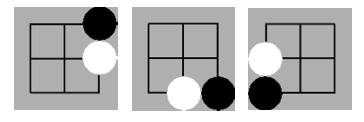
For example, game state below has same result as other three rotated
ones.
Game State 1
Other Rotated 3 States
{linenos
1 2 3 4 5 6 7 8 9 10 11 12 13 14 15 16 17
defsimilarStatus(self, status: Tuple[Tuple[int, ...]]) -> List[Tuple[Tuple[int, ...]]]: ret = [] rotatedS = status for _ inrange(4): rotatedS = self.rotate(rotatedS) ret.append(rotatedS) return ret
defrotate(self, status: Tuple[Tuple[int, ...]]) -> Tuple[Tuple[int, ...]]: N = len(status) board = [[ConnectNGame.AVAILABLE] * N for _ inrange(N)]
for r inrange(N): for c inrange(N): board[c][N - 1 - r] = status[r][c]
returntuple([tuple(board[i]) for i inrange(N)])
Minimax Strategy
Precomputation
In last version of Minimax DP strategy implementation, we searched
best game result given a game state. In the computation, we also
leveraged pruning to shortcut if the result is already best. However,
for AI agent, we still have to call minimax for each new game state
encountered. This is very inefficient because we are solving same game
states again and again during top down recursion. An obvious improvement
is to compute all game states in first step and cache them all. Later
for each given state encountered, we only need to aggregate result by
looking at all possible next move positions of that game state. Code of
aggregating possible moves is listed below.
defaction(self, game: ConnectNGame) -> Tuple[int, Tuple[int, int]]: game = copy.deepcopy(game)
player = game.currentPlayer bestResult = player * -1# assume opponent win as worst result bestMove = None for move in game.getAvailablePositions(): game.move(*move) status = game.getStatus() game.undo()
result = self.dpMap[status]
if player == ConnectNGame.PLAYER_A: bestResult = max(bestResult, result) else: bestResult = min(bestResult, result) # update bestMove if any improvement bestMove = move if bestResult == result else bestMove print(f'move {move} => {result}')
return bestResult, bestMove
Agent Class and Playing
Logic
We also construct Agent class hierarchy, allowing AI player and human
player to share common code.
BaseAgent is the root class with default act() method being making
random decisions over all available actions.
This episode extends last one, where Minimax and Alpha Beta Pruning
algorithms are introduced. We will solve several tic-tac-toe problems in
leetcode, gathering intuition and building blocks for tic-tac-toe game
logic, which can be naturally extended to Connect-N game or Gomoku
(N=5). Then we solve tic-tac-toe using Minimax and Alpha Beta pruning
for small N and analyze their state space. In the following episodes,
based on building blocks here, we will implement a Connect-N Open Gym
GUI Environment, where we can play against computer visually or compare
different computer algorithms. Finally, we demonstrate how to implement
a Monte Carlo Tree Search for Connect-N Game.
Tic-tac-toe is played by two players A and B on a 3 x 3 grid.
Here are the rules of Tic-Tac-Toe: Players take turns placing
characters into empty squares (" "). The first player A always
places "X" characters, while the second player B always places "O"
characters. "X" and "O" characters are always placed into empty
squares, never on filled ones. The game ends when there are 3 of
the same (non-empty) character filling any row, column, or
diagonal. The game also ends if all squares are non-empty. No
more moves can be played if the game is over. Given an array moves where
each element is another array of size 2 corresponding to the row and
column of the grid where they mark their respective character in the
order in which A and B play. Return the winner of the game if it
exists (A or B), in case the game ends in a draw return "Draw", if there
are still movements to play return "Pending". You can assume that
moves is valid (It follows the rules of Tic-Tac-Toe), the grid is
initially empty and A will play first.
Example 1: Input: moves = [[0,0],[2,0],[1,1],[2,1],[2,2]]
Output: "A" Explanation: "A" wins, he always plays first. "X "
"X " "X " "X " "X " " " -> " " -> " X " -> " X " -> " X
" " " "O " "O " "OO " "OOX"
Example 3: Input: moves =
[[0,0],[1,1],[2,0],[1,0],[1,2],[2,1],[0,1],[0,2],[2,2]] Output:
"Draw" Explanation: The game ends in a draw since there are no
moves to make. "XXO" "OOX" "XOX"
Example 4: Input: moves = [[0,0],[1,1]] Output:
"Pending" Explanation: The game has not finished yet. "X
" " O " " "
The intuitive solution is to permute all 8 possible winning
conditions: 3 vertical lines, 3 horizontal lines and 2 diagonal lines.
We keep 8 variables representing each winning condition and a simple
trick is converting board state to a 3x3 2d array, whose cell has value
-1, 1, and 0. In this way, we can traverse the board state exactly once
and in the process determine all 8 variables value by summing
corresponding cell value. For example, row[0] is for first line winning
condition, summed by all 3 cells in first row during board traveral. It
indicates win for first player only when it's equal to 3 and win for
second player when it's -3.
classSolution: deftictactoe(self, moves: List[List[int]]) -> str: board = [[0] * 3for _ inrange(3)] for idx, xy inenumerate(moves): player = 1if idx % 2 == 0else -1 board[xy[0]][xy[1]] = player
turn = 0 row, col = [0, 0, 0], [0, 0, 0] diag1, diag2 = False, False for r inrange(3): for c inrange(3): turn += board[r][c] row[r] += board[r][c] col[c] += board[r][c] if r == c: diag1 += board[r][c] if r + c == 2: diag2 += board[r][c]
oWin = any(row[r] == 3for r inrange(3)) orany(col[c] == 3for c inrange(3)) or diag1 == 3or diag2 == 3 xWin = any(row[r] == -3for r inrange(3)) orany(col[c] == -3for c inrange(3)) or diag1 == -3or diag2 == -3
Below we give another AC solution. Despite more code, it's more
efficient than previous one because for a given game state, it does not
need to visit each cell on the board. How is it achieved? The problem
guarentees each move is valid, so what's sufficent to examine is to
check neighbours of the final move and see if any line including final
move creates a winning condition. Later we will reuse the code in this
solution to create tic-tac-toe game logic.
if (north + south + 1 >= 3) or (east + west + 1 >= 3) or \ (south_east + north_west + 1 >= 3) or (north_east + south_west + 1 >= 3): returnTrue returnFalse
defgetConnectedNum(self, r: int, c: int, dr: int, dc: int) -> int: player = self.board[r][c] result = 0 i = 1 whileTrue: new_r = r + dr * i new_c = c + dc * i if0 <= new_r < 3and0 <= new_c < 3: if self.board[new_r][new_c] == player: result += 1 else: break else: break i += 1 return result
deftictactoe(self, moves: List[List[int]]) -> str: self.board = [[0] * 3for _ inrange(3)] for idx, xy inenumerate(moves): player = 1if idx % 2 == 0else -1 self.board[xy[0]][xy[1]] = player
# only check last move r, c = moves[-1] win = self.checkWin(r, c) if win: return"A"iflen(moves) % 2 == 1else"B"
A Tic-Tac-Toe board is given as a string array board. Return True if
and only if it is possible to reach this board position during the
course of a valid tic-tac-toe game. The board is a 3 x 3 array, and
consists of characters " ", "X", and "O". The " " character represents
an empty square. Here are the rules of Tic-Tac-Toe: Players
take turns placing characters into empty squares (" "). The first
player A always places "X" characters, while the second player B always
places "O" characters. "X" and "O" characters are always placed
into empty squares, never on filled ones. The game ends when there
are 3 of the same (non-empty) character filling any row, column, or
diagonal. The game also ends if all squares are non-empty. No
more moves can be played if the game is over.
Example 1: Input: board = ["O ", " ", " "] Output:
false Explanation: The first player always plays "X".
Example 2: Input: board = ["XOX", " X ", " "] Output:
false Explanation: Players take turns making moves.
Example 4: Input: board = ["XOX", "O O", "XOX"] Output:
true
Note: board is a length-3 array of strings, where each string
board[i] has length 3. Each board[i][j] is a character in the set
{" ", "X", "O"}.
Surely, it can be solved using DFS, checking if the state given would
be reached from initial state. However, this involves lots of states to
search. Could we do better? There are obvious properties we can rely on.
For example, the number of X is either equal to the number of O or one
more. If we can enumerate a combination of necessary and sufficient
conditions of checking its reachability, we can solve it in O(1) time
complexity.
Design a Tic-tac-toe game that is played between two players on a n x
n grid. You may assume the following rules: A move is
guaranteed to be valid and is placed on an empty block. Once a
winning condition is reached, no more moves is allowed. A player
who succeeds in placing n of their marks in a horizontal, vertical, or
diagonal row wins the game.
Example: Given n = 3, assume that player 1 is "X" and player 2
is "O" in the board. TicTacToe toe = new TicTacToe(3);
toe.move(0, 0, 1); -> Returns 0 (no one wins) |X| | | | | |
| // Player 1 makes a move at (0, 0). | | | |
toe.move(0, 2, 2); -> Returns 0 (no one wins) |X| |O| | | |
| // Player 2 makes a move at (0, 2). | | | |
toe.move(2, 2, 1); -> Returns 0 (no one wins) |X| |O| | | |
| // Player 1 makes a move at (2, 2). | | |X|
toe.move(1, 1, 2); -> Returns 0 (no one wins) |X| |O| | |O|
| // Player 2 makes a move at (1, 1). | | |X|
toe.move(2, 0, 1); -> Returns 0 (no one wins) |X| |O| | |O|
| // Player 1 makes a move at (2, 0). |X| |X|
toe.move(1, 0, 2); -> Returns 0 (no one wins) |X| |O| |O|O|
| // Player 2 makes a move at (1, 0). |X| |X|
toe.move(2, 1, 1); -> Returns 1 (player 1 wins) |X| |O|
|O|O| | // Player 1 makes a move at (2, 1). |X|X|X|
Follow up: Could you do better than O(n2) per move()
operation?
348 is a locked problem. For each player's move, we can resort to
checkWin function in second solution for 1275. We show another solution
based on first solution of 1275, where 8 winning condition flags are
kept and each move only touches associated several flag variables.
def__init__(self, n:int): """ Initialize your data structure here. :type n: int """ self.row, self.col, self.diag1, self.diag2, self.n = [0] * n, [0] * n, 0, 0, n
defmove(self, row:int, col:int, player:int) -> int: """ Player {player} makes a move at ({row}, {col}). @param row The row of the board. @param col The column of the board. @param player The player, can be either 1 or 2. @return The current winning condition, can be either: 0: No one wins. 1: Player 1 wins. 2: Player 2 wins. """ if player == 2: player = -1
self.row[row] += player self.col[col] += player if row == col: self.diag1 += player if row + col == self.n - 1: self.diag2 += player
if self.n in [self.row[row], self.col[col], self.diag1, self.diag2]: return1 if -self.n in [self.row[row], self.col[col], self.diag1, self.diag2]: return2 return0
Optimal Strategy of
Tic-Tac-Toe
Tic-tac-toe and Gomoku (Connect Five in a Row) share the same rules
and are generally considered as M,n,k-game, where
board size range to M x N and winning condition changes to k.
ConnectNGame class implements M,n,k-game of MxM board size. It
encapsulates the logic of checking each move and also is able to undo
last move to facilitate backtrack in game search algorithm later.
defgetAvailablePositions(self) -> List[Tuple[int, int]]: return [(i,j) for i inrange(self.board_size) for j inrange(self.board_size) if self.board[i][j] == ConnectNGame.AVAILABLE]
defgetStatus(self) -> Tuple[Tuple[int, ...]]: returntuple([tuple(self.board[i]) for i inrange(self.board_size)])
Note that checkWin code is identical to second solution in 1275.
Minimax Strategy
Now we have Connect-N game logic, let's finish its minimax algorithm
to solve the game.
Define a generic strategy base class, where action method needs to be
overridden. Action method expects ConnectNGame class telling current
game state and returns a tuple of 2 elements, the first element is the
estimated or exact game result after taking action specified by second
element. The second element is of form Tuple[int, int], denoting the
position of the move, for instance, (1,1).
defminimax(self) -> Tuple[int, Tuple[int, int]]: game = self.game bestMove = None assertnot game.gameOver if game.currentPlayer == ConnectNGame.PLAYER_A: ret = -math.inf for pos in game.getAvailablePositions(): move = pos result = game.move(*pos) if result isNone: assertnot game.gameOver result, oppMove = self.minimax() game.undo() ret = max(ret, result) bestMove = move if ret == result else bestMove if ret == 1: return1, move return ret, bestMove else: ret = math.inf for pos in game.getAvailablePositions(): move = pos result = game.move(*pos) if result isNone: assertnot game.gameOver result, oppMove = self.minimax() game.undo() ret = min(ret, result) bestMove = move if ret == result else bestMove if ret == -1: return -1, move return ret, bestMove
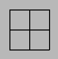
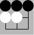
We plot up to first 2 moves with code above. For first
player O, there are possibly 9 positions, where due to symmetry, only 3
kinds of moves, which we call corner, edge and center, respectively. The
following graph shows whatever 9 positions the first player takes, the
best result is draw. So solution of tic-tac-toe is draw.
Tic-tac-toe 9 First Step
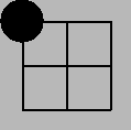
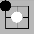
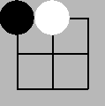
Plot first step of 3 kinds of moves one by one below.
Tic-tac-toe First Step Corner
Tic-tac-toe First Step Edge
Tic-tac-toe First Step Center
Tic-tac-toe Solution
and Number of States
An interesting question is the number of game states of tic-tac-toe.
A loosely upper bound can be derived by \(3^9=19683\), which includes lots of
inreachable states. This article Tic-Tac-Toe
(Naughts and Crosses, Cheese and Crackers, etc lists number of
states after each move. The total number is 5478.
Moves
Positions
Terminal Positions
0
1
1
9
2
72
3
252
4
756
5
1260
120
6
1520
148
7
1140
444
8
390
168
9
78
78
Total
5478
958
We can verify the number if we change a little of existing code to
code below.
if gameStatus in self.dpMap: return self.dpMap[gameStatus]
game = self.game bestMove = None assertnot game.gameOver if game.currentPlayer == ConnectNGame.PLAYER_A: ret = -math.inf for pos in game.getAvailablePositions(): move = pos result = game.move(*pos) if result isNone: assertnot game.gameOver result, oppMove = self.minimax(game.getStatus()) self.dpMap[game.getStatus()] = result, oppMove else: self.dpMap[game.getStatus()] = result, move game.undo() ret = max(ret, result) bestMove = move if ret == result else bestMove self.dpMap[gameStatus] = ret, bestMove return ret, bestMove else: ret = math.inf for pos in game.getAvailablePositions(): move = pos result = game.move(*pos)
if result isNone: assertnot game.gameOver result, oppMove = self.minimax(game.getStatus()) self.dpMap[game.getStatus()] = result, oppMove else: self.dpMap[game.getStatus()] = result, move game.undo() ret = min(ret, result) bestMove = move if ret == result else bestMove self.dpMap[gameStatus] = ret, bestMove return ret, bestMove
if __name__ == '__main__': tic_tac_toe = ConnectNGame(N=3, board_size=3) strategy = CountingMinimaxStrategy() strategy.action(tic_tac_toe) print(f'Game States Number {len(strategy.dpMap)}')
Running the code proves the total number is 5478. Also illustrate
some small scale game configuration results.
3x3
4x4
k=3
5478 (Draw)
6035992 (Win)
k=4
9722011 (Draw)
k=5
According to Wikipedia
M,n,k-game, below are results for some game configuration.
3x3
4x4
5x5
6x6
k=3
Draw
Win
Win
Win
k=4
Draw
Draw
Win
k=5
Draw
Draw
What's worth mentioning is that Gomoku (Connect Five in a Row), of
board size MxM >= 15x15 is proved by L. Victor Allis to be Win.
defalpha_beta(self, gameStatus: Tuple[Tuple[int, ...]], alpha:int=None, beta:int=None) -> Tuple[int, Tuple[int, int]]: game = self.game bestMove = None assertnot game.gameOver if game.currentPlayer == ConnectNGame.PLAYER_A: ret = -math.inf for pos in game.getAvailablePositions(): move = pos result = game.move(*pos) if result isNone: assertnot game.gameOver result, oppMove = self.alpha_beta(game.getStatus(), alpha, beta) game.undo() alpha = max(alpha, result) ret = max(ret, result) bestMove = move if ret == result else bestMove if alpha >= beta or ret == 1: return ret, move return ret, bestMove else: ret = math.inf for pos in game.getAvailablePositions(): move = pos result = game.move(*pos) if result isNone: assertnot game.gameOver result, oppMove = self.alpha_beta(game.getStatus(), alpha, beta) game.undo() beta = min(beta, result) ret = min(ret, result) bestMove = move if ret == result else bestMove if alpha >= beta or ret == -1: return ret, move return ret, bestMove
Rewrite alpha beta pruning with DP, where we omit alpha and beta
parameters in alpha_beta_dp because lru_cache cannot specify effective
parameters. Instead, we keep alpha and beta in a stack variable and
maintain the stack according to alpha_bate_dp calling stack.
@lru_cache(maxsize=None) defalpha_beta_dp(self, gameStatus: Tuple[Tuple[int, ...]]) -> Tuple[int, Tuple[int, int]]: alpha, beta = self.alphaBetaStack[-1] game = self.game bestMove = None assertnot game.gameOver if game.currentPlayer == ConnectNGame.PLAYER_A: ret = -math.inf for pos in game.getAvailablePositions(): move = pos result = game.move(*pos) if result isNone: assertnot game.gameOver self.alphaBetaStack.append((alpha, beta)) result, oppMove = self.alpha_beta_dp(game.getStatus()) self.alphaBetaStack.pop() game.undo() alpha = max(alpha, result) ret = max(ret, result) bestMove = move if ret == result else bestMove if alpha >= beta or ret == 1: return ret, move return ret, bestMove else: ret = math.inf for pos in game.getAvailablePositions(): move = pos result = game.move(*pos) if result isNone: assertnot game.gameOver self.alphaBetaStack.append((alpha, beta)) result, oppMove = self.alpha_beta_dp(game.getStatus()) self.alphaBetaStack.pop() game.undo() beta = min(beta, result) ret = min(ret, result) bestMove = move if ret == result else bestMove if alpha >= beta or ret == -1: return ret, move return ret, bestMove
This series, we deal with zero-sum turn-based board game algorithm, a
sub type of combinatorial games. We start off with small search space
problem, introduce classic algorithms and corresponding combinatorial
gaming theory and ultimately end with modern approximating Deep RL
techniques. From there, after stepping stone is laid, we are able to
learn and appreciate how AlphaGo works. In this first episode, we
illustrate 3 classic gaming problems in leetcode and solve them from
brute force version to DP version then finally rewrite them using
classic gaming algorithms, minimax and alpha beta pruning.
You are playing the following Nim Game with your friend: There is a
heap of stones on the table, each time one of you take turns to remove 1
to 3 stones. The one who removes the last stone will be the winner. You
will take the first turn to remove the stones. Both of you are very
clever and have optimal strategies for the game. Write a function to
determine whether you can win the game given the number of stones in the
heap.
Example: Input: 4 Output: false Explanation: If there
are 4 stones in the heap, then you will never win the game; No
matter 1, 2, or 3 stones you remove, the last stone will always be
removed by your friend.
Let \(f(n)\) be the result, either
Win or Lose, when you take turn to make optimal move for the case of
\(n\) stones. The first non trial case
is \(f(4)\). By playing optimal
strategies, it is equivalent to saying if there is any chance that leads
to Win, you will definitely choose it. So you try 1, 2, 3 stones and see
whether your opponent has any chance to win. Obviously, \(f(1) = f(2) = f(3) = Win\). Therefore,
\(f(4)\) is guranteed to lose.
Generally, the recurrence relation is given by \[
f(n) = \neg (f(n-1) \land f(n-2) \land f(n-3))
\]
This translates straightforwardly to following Python 3 code.
{linenos
1 2 3 4 5 6 7 8 9 10 11
# TLE # Time Complexity: O(exponential) classSolution_BruteForce:
defcanWinNim(self, n: int) -> bool: if n <= 3: returnTrue for i inrange(1, 4): ifnot self.canWinNim(n - i): returnTrue returnFalse
Since this brute force version has same recursive manner
as fibonacci number, the complexity is exponential so it won't pass
test. This can be visually verified by following call graph. Notice,
node 5 is expanded entirely twice and node 4 is expanded 4 times.
292 Nim Game Brute Force Call Graph, n=7
As what we optimize for computing fibonacci, we cache the result for
smaller number and compute larger value based on previous ones. In
Python, we can achieve the DP cache effect by merely adding one line,
the magical decorator lru_cache. In this way, runtime
complexity is drastically reduced to \(O(N)\).
{linenos
1 2 3 4 5 6 7 8 9 10 11 12
# RecursionError: maximum recursion depth exceeded in comparison n=1348820612 # Time Complexity: O(N) classSolution_DP: from functools import lru_cache @lru_cache(maxsize=None) defcanWinNim(self, n: int) -> bool: if n <= 3: returnTrue for i inrange(1, 4): ifnot self.canWinNim(n - i): returnTrue returnFalse
Plotting the call
graph below helps to verify that. This time, node 5 and 4 are not
explored to bottom multiple times. The green node denotes such cache
hit.
292 Nim Game DP Call Graph, n=7
However, for this problem, lru_cache is not enough to AC because for
large n, such as 1348820612, the implementation suffers from stack
overflow. We can, of course, rewrite it in iterative forwarding loop
manner. But still TLE.
{linenos
1 2 3 4 5 6 7 8 9 10 11
# TLE for 1348820612 # Time Complexity: O(N) classSolution: defcanWinNim(self, n: int) -> bool: if n <= 3: returnTrue last3, last2, last1 = True, True, True for i inrange(4, n+1): this = not (last3 and last2 and last1) last3, last2, last1 = last2, last1, this return last1
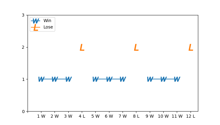
So AC code requires at most sublinear complexity. The last version
also gives us some intuition that win lose may have period of 4.
Actually, if you arrange all \(f(n)\)
one by one, it's obvious that any \(n \mod 4 =
0\) leads to Lose and other cases lead to Win. Why? Suppose you
start with \(4k+i (i=1,2,3)\), you can
always remove \(i\) stones and leave
\(4k\) stones to your opponent.
Whatever he chooses, you are returned with situation \(4k_1 + i_1 (i_1 = 1,2,3)\). This pattern
repeats until you have 1, 2, 3 remaining stones.
Win Lose Distribution
Below is one liner AC version.
{linenos
1 2 3 4 5
# AC # Time Complexity: O(1) classSolution: defcanWinNim(self, n: int) -> bool: returnnot (n % 4 == 0)
Given an array of scores that are non-negative integers. Player 1
picks one of the numbers from either end of the array followed by the
player 2 and then player 1 and so on. Each time a player picks a number,
that number will not be available for the next player. This continues
until all the scores have been chosen. The player with the maximum score
wins. Given an array of scores, predict whether player 1 is the
winner. You can assume each player plays to maximize his score.
Example 1: Input: [1, 5, 2] Output: False
Explanation: Initially, player 1 can choose between 1 and 2. If he
chooses 2 (or 1), then player 2 can choose from 1 (or 2) and 5. If
player 2 chooses 5, then player 1 will be left with 1 (or 2). So,
final score of player 1 is 1 + 2 = 3, and player 2 is 5. Hence,
player 1 will never be the winner and you need to return False.
Example 2: Input: [1, 5, 233, 7] Output: True
Explanation: Player 1 first chooses 1. Then player 2 have to choose
between 5 and 7. No matter which number player 2 choose, player 1 can
choose 233. Finally, player 1 has more score (234) than player 2
(12), so you need to return True representing player1 can win.
For a player, he can choose leftmost or rightmost one and leave
remaining array to his opponent. Let us define maxDiff(l, r) to be the
maximum difference current player can get, who is facing situation of
subarray \([l, r]\).
Exponential runtime complexity can also be verified by call graph below.
486 Predict the Winner Brute Force Call Graph, n=4
Again, be aware we have repeated computation over same node, for
example, [1-2] node is expanded entirely for the second time when going
from root to right node. Applying the same lru_cache trick, the one
liner decorating maxDiff, we passed again with runtime complexity \(O(n^2)\) and running time 43ms, trial
change but substantial improvement!
{linenos
1
2
3
4
5
6
7
8
9
10
11
12
13
14
15
16
17
# AC # Time Complexity: O(N^2) # Fast: 43ms from functools import lru_cache from typing importList
classSolution:
@lru_cache(maxsize=None) defmaxDiff(self, l: int, r:int) -> int: if l == r: return self.nums[l] returnmax(self.nums[l] - self.maxDiff(l + 1, r), self.nums[r] - self.maxDiff(l, r - 1))
Taking look at DP version call graph, this time, [1-2] node is not
re-computed in right branch.
486 Predict the Winner DP Call Graph, n=4
Leetcode 464 Can I Win
(Medium)
A similar but slightly difficult problem is Leetcode 464 Can I
Win, where bit mask with DP technique is employed.
In the "100 game," two players take turns adding, to a running total,
any integer from 1..10. The player who first causes the running total to
reach or exceed 100 wins. What if we change the game so that
players cannot re-use integers? For example, two players might take
turns drawing from a common pool of numbers of 1..15 without replacement
until they reach a total >= 100. Given an integer
maxChoosableInteger and another integer desiredTotal, determine if the
first player to move can force a win, assuming both players play
optimally. You can always assume that maxChoosableInteger will not
be larger than 20 and desiredTotal will not be larger than 300.
Example Input: maxChoosableInteger = 10 desiredTotal =
11 Output: false Explanation: No matter which
integer the first player choose, the first player will lose. The
first player can choose an integer from 1 up to 10. If the first
player choose 1, the second player can only choose integers from 2 up to
10. The second player will win by choosing 10 and get a total = 11,
which is >= desiredTotal. Same with other integers chosen by the
first player, the second player will always win.
Because there are \(2^m\) states and
for each state we need to probe at most \(m\) options, so the overall runtime
complexity is \(O(m 2^m)\), where m is
maxChoosableInteger.
Minimax Algorithm
Up till now, we've seen serveral zero-sum turn based gaming in
leetcode. In fact, there is more general algorithm for this type of
gaming, named, minimax algorithm with alternate moves. The general
setting is that, two players play in turn. The first player is trying to
maximize game value and second player trying to minimize game value. For
example, the following graph shows all nodes, labelled by its value.
Computing from bottom up, the first player (max) can get optimal value
-7, assuming both players play optimially.
Wikipedia Minimax Example
Pseudo code in Python 3 is listed below.
{linenos
1 2 3 4 5 6 7 8 9 10 11 12 13
defminimax(node: Node, depth: int, maximizingPlayer: bool) -> int: if depth == 0or is_terminal(node): return evaluate_terminal(node) if maximizingPlayer: value:int = −∞ for child in node: value = max(value, minimax(child, depth − 1, False)) return value else: # minimizing player value := +∞ for child in node: value = min(value, minimax(child, depth − 1, True)) return value
Minimax: 486 Predict the
Winner
We know leetcode 486 Predict the Winner is zero-sum turn-based game.
Hence, theoretically, we can come up with a minimax algorithm for it.
But the difficulty lies in how we define value or utility for it. In
previous section, we've defined maxDiff(l, r) to be the maximum
difference for current player, who is left with sub array \([l, r]\). In the most basic case, where
only one element x is left, it's intuitive to define +x for max player
and -x for min player. If we merge it with minimax algorithm, it's
naturally follows that, the total reward got by max player is \(+a_1 + a_2 + ... = A\) and reward by min
player is \(-b_1 - b_2 - ... = -B\),
and max player aims to \(max(A-B)\)
while min player aims to \(min(A-B)\).
With that in mind, code is not hard to implement.
# AC from functools import lru_cache from typing importList
classSolution: # max_player: max(A - B) # min_player: min(A - B) @lru_cache(maxsize=None) defminimax(self, l: int, r: int, isMaxPlayer: bool) -> int: if l == r: return self.nums[l] * (1if isMaxPlayer else -1)
if isMaxPlayer: returnmax( self.nums[l] + self.minimax(l + 1, r, not isMaxPlayer), self.nums[r] + self.minimax(l, r - 1, not isMaxPlayer)) else: returnmin( -self.nums[l] + self.minimax(l + 1, r, not isMaxPlayer), -self.nums[r] + self.minimax(l, r - 1, not isMaxPlayer))
defPredictTheWinner(self, nums: List[int]) -> bool: self.nums = nums v = self.minimax(0, len(nums) - 1, True) return v >= 0
Minimax 486 Case [1, 5, 2, 4]
Minimax: 464 Can I Win
For this problem, as often processed in other win-lose-tie game
without intermediate intrinsic value, it's typically to define +1 in
case max player wins, -1 for min player and 0 for tie. Note the shortcut
case for both player. For example, the max player can report Win
(value=1) once he finds winning condition (>=desiredTotal) is
satisfied during enumerating possible moves he can make. This also makes
sense since if he gets 1 during maxing, there can not be other value for
further probing that is finally returned. The same optimization will be
generalized in the next improved algorithm, alpha beta pruning.
# AC classSolution: from functools import lru_cache @lru_cache(maxsize=None) # currentTotal < desiredTotal defminimax(self, status: int, currentTotal: int, isMaxPlayer: bool) -> int: import math if status == self.allUsed: return0# draw: no winner
if isMaxPlayer: value = -math.inf for i inrange(1, self.maxChoosableInteger + 1): ifnot (status >> i & 1): new_status = 1 << i | status if currentTotal + i >= self.desiredTotal: return1# shortcut value = max(value, self.minimax(new_status, currentTotal + i, not isMaxPlayer)) if value == 1: return1 return value else: value = math.inf for i inrange(1, self.maxChoosableInteger + 1): ifnot (status >> i & 1): new_status = 1 << i | status if currentTotal + i >= self.desiredTotal: return -1# shortcut value = min(value, self.minimax(new_status, currentTotal + i, not isMaxPlayer)) if value == -1: return -1 return value
Alpha-Beta Pruning
We sensed there is space of optimaization during searching, as
illustrated in 464 Can I Win minimax algorithm. Let's formalize this
idea, called alpha beta pruning. For each node, we maintain two values
alpha and beta, which represent the minimum score that the maximizing
player is assured of and the maximum score that the minimizing player is
assured of, respectively. The root node has initial alpha = −∞ and beta
= +∞, forming valid duration [−∞, +∞]. During top down traversal, child
node inherits alpha beta value from its parent node, for example,
[alpha, beta], if the updated alpha or beta in the child node no longer
forms a valid interval, the branch can be pruned and return immediately.
Take following example in Wikimedia for example.
Root node, intially: alpha = −∞, beta = +∞
Root node, after 4 is returned, alpha = 4, beta = +∞
Root node, after 5 is returned, alpha = 5, beta = +∞
Rightmost Min node, intially: alpha = 5, beta = +∞
Rightmost Min node, after 1 is returned: alpha = 5, beta =
1
Here we see [5, 1] no longer is valid interval, so it returns without
further probing his 2nd and 3rd child. Why? because if the other child
returns value > 1, say 2, it will be replaced by 1 as it's a min node
with guarenteed value 1. If the other child returns value < 1, it
will be abandoned by root node, a max node, which has already guarenteed
to have value >=5. So in this situation, whatever other children
return does not impact anything.
Wikimedia Alpha Beta Pruning Example
Pseudo code in Python 3 is listed below.
{linenos
1 2 3 4 5 6 7 8 9 10 11 12 13 14 15 16 17 18 19
defalpha_beta(node: Node, depth: int, α: int, β: int, maximizingPlayer: bool) -> int: if depth == 0or is_terminal(node): return evaluate_terminal(node) if maximizingPlayer: value: int = −∞ for child in node: value = max(value, alphabeta(child, depth − 1, α, β, False)) α = max(α, value) if α >= β: break# β cut-off return value else: value: int = +∞ for child in node: value = min(value, alphabeta(child, depth − 1, α, β, True)) β = min(β, value) if β <= α: break# α cut-off return value
# AC classSolution: from functools import lru_cache @lru_cache(maxsize=None) # currentTotal < desiredTotal defalpha_beta(self, status: int, currentTotal: int, isMaxPlayer: bool, alpha: int, beta: int) -> int: import math if status == self.allUsed: return0# draw: no winner
if isMaxPlayer: value = -math.inf for i inrange(1, self.maxChoosableInteger + 1): ifnot (status >> i & 1): new_status = 1 << i | status if currentTotal + i >= self.desiredTotal: return1# shortcut value = max(value, self.alpha_beta(new_status, currentTotal + i, not isMaxPlayer, alpha, beta)) alpha = max(alpha, value) if alpha >= beta: return value return value else: value = math.inf for i inrange(1, self.maxChoosableInteger + 1): ifnot (status >> i & 1): new_status = 1 << i | status if currentTotal + i >= self.desiredTotal: return -1# shortcut value = min(value, self.alpha_beta(new_status, currentTotal + i, not isMaxPlayer, alpha, beta)) beta = min(beta, value) if alpha >= beta: return value return value
C++, Java,
Javascript for 486 Predict the Winner
As a bonus, we AC leetcode 486 in C++, Java and Javascript with a
bottom up iterative DP. We illustrate this method for other languages
not just because lru_cache is available in non Python languages, but
also because there are other ways to solve the problem. Notice the
topological ordering of DP dependency, building larger DP based on
smaller and solved ones. In addition, it's worth mentioning that this
approach is guaranteed to have \(n^2\)
loops but top down caching approach can have sub \(n^2\) loops.
Java AC Code
{linenos
1 2 3 4 5 6 7 8 9 10 11 12 13 14 15 16 17 18 19
// AC classSolution{ publicbooleanPredictTheWinner(int[] nums){ int n = nums.length; int[][] dp = newint[n][n]; for (int i = 0; i < n; i++) { dp[i][i] = nums[i]; }
for (int l = n - 1; l >= 0; l--) { for (int r = l + 1; r < n; r++) { dp[l][r] = Math.max( nums[l] - dp[l + 1][r], nums[r] - dp[l][r - 1]); } } return dp[0][n - 1] >= 0; } }
C++ AC Code
{linenos
1 2 3 4 5 6 7 8 9 10 11 12 13 14 15 16 17
// AC classSolution { public: boolPredictTheWinner(vector<int>& nums){ int n = nums.size(); vector<vector<int>> dp(n, vector<int>(n, 0)); for (int i = 0; i < n; i++) { dp[i][i] = nums[i]; } for (int l = n - 1; l >= 0; l--) { for (int r = l + 1; r < n; r++) { dp[l][r] = max(nums[l] - dp[l + 1][r], nums[r] - dp[l][r - 1]); } } return dp[0][n - 1] >= 0; } };
for (let i = 0; i < n; i++) { dp[i][i] = nums[i]; } for (let l = n - 1; l >=0; l--) { for (let r = i + 1; r < n; r++) { dp[l][r] = Math.max(nums[l] - dp[l + 1][r],nums[r] - dp[l][r - 1]); } } return dp[0][n-1] >=0; };
This is fifth episode of series: TSP From DP to Deep Learning. In
this episode, we turn to Reinforcement Learning technology, in
particular, a model-free policy gradient method that embeds pointer
network to learn minimal tour without supervised best tour label in
dataset. Full list of this series is listed below.
The stochastic policy \(p(\pi | s;
\theta)\), parameterized by \(\theta\), is aiming to assign high
probabilities to short tours and low probabilities to long tours. The
joint probability assumes independency to allow factorization.
The loss of the model is cross entropy between the network’s output
probabilities \(\pi\) and the best tour
\(\hat{\pi}\) generated by a TSP
solver.
Contribution made by Pointer networks is that it addressed the
constraint in that it allows for dynamic index value given by the
particular test case, instead of from a fixed-size vocabulary.
Reinforcement Learning
Neural Combinatorial Optimization with Reinforcement Learning
combines the power of Reinforcement Learning (RL) and Deep
Learning to further eliminate the constraint required by Pointer
Networks that the training dataset has to have supervised labels of best
tour. With deep RL, test cases do not need to have a solution which is
common pattern in deep RL. In the paper, a model-free policy-based RL
method is adopted.
Model-Free Policy Gradient
Methods
In the authoritative RL book, chapter 8 Planning and Learning
with Tabular Methods, there are two major approaches in RL. One is
model-based RL and the other is model-free RL. Distinction between the
two relies on concept of model, which is stated as follows:
By a model of the environment we mean anything that an agent can use
to predict how the environment will respond to its actions.
So model-based methods demand a model of the environment, and hence
dynamic programming and heuristic search fall into this category. With
model in mind, utility of the state can be computed in various ways and
planning stage that essentially builds policy is needed before agent can
take any action. In contrast, model-free methods, without building a
model, are more direct, ignoring irrelevant information and just
focusing on the policy which is ultimately needed. Typical examples of
model-free methods are Monte Carlo Control and Temporal-Difference
Learning. >Model-based methods rely on planning as their primary
component, while model-free methods primarily rely on learning.
In TSP problem, the model is fully determined by all points given,
and no feedback is generated for each decision made. So it's unclear to
how to map state value with a tour. Therefore, we turn to model-free
methods. In chapter 13 Policy Gradient Methods, a particular
approximation model-free method that learns a parameterized policy that
can select actions without consulting a value function. This approach
fits perfectly with aforementioned pointer networks where the
parameterized policy \(p(\pi | s;
\theta)\) is already defined.
Training objective is obvious, the expected tour length of \(\pi_\theta\) which, given an input graph
\(s\)
Monte Carlo
Policy Gradient: REINFORCE with Baseline
In order to find largest reward, a typical way is to optimize the
parameters \(\theta\) in the direction
of derivative: \(\nabla_{\theta} J(\theta |
s)\).
RHS of equation above is the derivative of expectation that we have
no idea how to compute or approximate. Here comes the well-known
REINFORCE trick that turns it into form of expectation of derivative,
which can be approximated easily with Monte Carlo sampling, where the
expectation is replaced by averaging.
Another common trick, subtracting a baseline \(b(s)\), leads the derivative of reward to
the following equation. Note that \(b(s)\) denotes a baseline function that
must not depend on \(\pi\). \[
\nabla_{\theta} J(\theta | s)=\mathbb{E}_{\pi \sim p_{\theta}(. |
s)}\left[(L(\pi | s)-b(s)) \nabla_{\theta} \log p_{\theta}(\pi |
s)\right]
\]
The trick is explained in as:
Because the baseline could be uniformly zero, this update is a strict
generalization of REINFORCE. In general, the baseline leaves the
expected value of the update unchanged, but it can have a large effect
on its variance.
Finally, the equation can be approximated with Monte Carlo sampling,
assuming drawing \(B\) i.i.d: \(s_{1}, s_{2}, \ldots, s_{B} \sim
\mathcal{S}\) and sampling a single tour per graph: $ {i}
p{}(. | s_{i}) $, as follows \[
\nabla_{\theta} J(\theta) \approx \frac{1}{B}
\sum_{i=1}^{B}\left(L\left(\pi_{i} |
s_{i}\right)-b\left(s_{i}\right)\right) \nabla_{\theta} \log
p_{\theta}\left(\pi_{i} | s_{i}\right)
\]
Actor Critic Methods
REINFORCE with baseline works quite well but it also has
disadvantage.
REINFORCE with baseline is unbiased and will converge asymptotically
to a local minimum, but like all Monte Carlo methods it tends to learn
slowly (produce estimates of high variance) and to be inconvenient to
implement online or for continuing problems.
A typical improvement is actor–critic methods, that not only learn
approximate policy, the actor job, but also learn approximate value
funciton, the critic job. This is because it reduces variance and
accelerates learning via a bootstrapping critic that introduce bias
which is often beneficial. Detailed algorithm in the paper illustrated
below.
defforward(self, batch_input: Tensor) -> Tuple[Tensor, List[Tensor], List[Tensor], List[Tensor]]: """ Args: batch_input: [batch_size * 2 * seq_len] Returns: R: Tensor of shape [batch_size] action_prob_list: List of [seq_len], tensor shape [batch_size] action_list: List of [seq_len], tensor shape [batch_size * 2] action_idx_list: List of [seq_len], tensor shape [batch_size] """ batch_size = batch_input.size(0) seq_len = batch_input.size(2) prob_list, action_idx_list = self.actor(batch_input)
action_list = [] batch_input = batch_input.transpose(1, 2) for action_id in action_idx_list: action_list.append(batch_input[[x for x inrange(batch_size)], action_id.data, :]) action_prob_list = [] for prob, action_id inzip(prob_list, action_idx_list): action_prob_list.append(prob[[x for x inrange(batch_size)], action_id.data])
R = self.reward(action_list)
return R, action_prob_list, action_list, action_idx_list defreward(self, sample_solution: List[Tensor]) -> Tensor: """ Computes total distance of tour Args: sample_solution: list of size N, each tensor of shape [batch_size * 2] Returns: tour_len: [batch_size] """ batch_size = sample_solution[0].size(0) n = len(sample_solution) tour_len = Variable(torch.zeros([batch_size]))
This is fourth episode of series: TSP From DP to Deep Learning. In
this episode, we systematically compare different searching algorithms
for finding most likely sequence in the context of simplied markov chain
setting. These models can be further utilized in deep learning decoding
stage, which will be illustrated in reinforcement learning, in the next
episode. Full list of this series is listed below.
In sequence-to-sequence problem, we are always faced with same
problem of determining the best or most likely sequence of output. This
kind of recurring problem exists extensively in algorithms, machine
learning where we are given initial states and the dynamics of the
system, and the goal is to find a path that is most likely. The
corresponding concept, in science or mathematical discipline, is called
Markov Chain.
Let describe the problem in the context of markov chain. Suppose
there are \(n\) states, and initial
state is given by $s_0 = [0.35, 0.25, 0.4] $. The transition matrix is
defined by \(T\) where $ T[i][j]$
denotes the probability of transitioning from \(i\) to \(j\). Notice that each row sums to \(1.0\). \[
T=
\begin{matrix}
& \begin{matrix}0&1&2\end{matrix} \\\\
\begin{matrix}0\\\\1\\\\2\end{matrix} &
\begin{bmatrix}0.3&0.6&0.1\\\\0.4&0.2&0.4\\\\0.3&0.3&0.4\end{bmatrix}\\\\
\end{matrix}
\]
Probability of the next state \(s_1\) is derived by multiplication of \(s_0\) and \(T\), which can be visually interpreted by
animation below.
The actual probability distribution value of \(s_1\) is computed numerically below. Recall
that left multiplying a row with a matrix amounts to making a linear
combination of that row vector.
\[
s_1 = \begin{bmatrix}0.35& 0.25& 0.4\end{bmatrix}
\begin{matrix}
\begin{bmatrix}0.3&0.6&0.1\\\\0.4&0.2&0.4\\\\0.3&0.3&0.4\end{bmatrix}\\\\
\end{matrix}
= \begin{bmatrix}0.325& 0.35& 0.255\end{bmatrix}
\] Again, state \(s_2\) can be
derived in the same way \(s_1 \times
T\), where we assume the transitioning dynamics remains the same.
However, in deep learning problem, the dynamics usually depends on \(s_i\), or vary according to the stage.
Suppose there are only 3 stages in our problem, e.g., \(s_0 \rightarrow s_1 \rightarrow s_2\). Let
\(L\) be the number of stages and \(N\) be the number of vertices in each
stage. Hence \(L=N=3\) in our problem
setting. There could be \(N^L\)
different paths starting from initial stage and to final stage.
Let us compute an arbitrary path probability as an example, \(2(s_0) \rightarrow 1(s_1) \rightarrow
2(s_2)\). The total probability is
First, we implement \(N^L\)
exhaustive or brute force search.
The following Python 3 function returns one most likely sequence and
its probability. Running the algorithm with our example produces 0.084
and route \(0 \rightarrow 1 \rightarrow
2\).
max_prop = 0.0 max_route = None prob = 0.0 for path inlist(path_all): for idx, v inenumerate(path): if idx == 0: prob = initial[v] # reset to initial state else: prev_v = path[idx-1] prob *= transition[prev_v][v] if prob > max_prop: max_prop = max(max_prop, prob) max_route = path return max_prop, max_route
Greedy Search
Exhaustive search always generates most likely sequence, as searching
for a needle in the hay at the cost of exponential runtime complexity
\(O(N^L)\). The simplest strategy,
unknown as greedy, identifies one vertex in each stage and then expand
the vertex in next stage. This strategy, of course, is not guaranteed to
find most likely sequence but is fast. See animation below.
Code in Python 3 is given below. Numpy package is employed to utilize
np.argmax() for code clarity. Notice there are 2 for loops (the other is
np.argmax) so the runtime complexity is \(O(N\times L)\).
prev_max_v = None for l inrange(0, L): max_v = np.argmax(states) max_route.append(max_v) if l == 0: max_prop = initial[max_v] else: max_prop = max_prop * transition[prev_max_v][max_v] states = max_prop * states prev_max_v = max_v
return max_prop, max_route
Beam Search
We could improve greedy strategy a little bit by expanding more
vertices in each stage. In beam search with \(k\) nodes, the strategy is in each stage,
identify \(k\) nodes with highest
probability and expand these \(k\)
nodes into next stage. In our example, \(k=2\), we select first 2 nodes in stage
\(s_0\), expand these 2 nodes and
evaluate \(2 \times 3\) nodes in stage
\(s_1\), then select 2 nodes and
evaluate 6 nodes in stage \(s_2\). Beam
search, similar to greedy strategy, is not guaranteed to find most
likely sequence but it extends search space with linear complexity.
Below is implementation in Python 3 with PriorityQueue to select top
\(k\) nodes. Notice in order to use
reverse order of PriorityQueue, a class with @total_ordering is required to be
defined. The runtime complexity is \(O(k\times
N \times L)\) .
for v inrange(N): next_q.put(PQItem(initial[v], str(v)))
for l inrange(1, L): current_q = next_q next_q = PriorityQueue() k = K whilenot current_q.empty() and k > 0: item = current_q.get() prob, route, prev_v = item.prob, item.route, item.last_v k -= 1 for v inrange(N): nextItem = PQItem(prob * transition[prev_v][v], route + str(v)) next_q.put(nextItem)
Similarly to TSP DP version, there is a dynamic programming approach,
widely known as Viterbi algorithm, that always finds out sequence with
max probability while reducing runtime complexity from \(O(N^L)\) to \(O(L
\times N \times N)\) (corresponding to 3 loops in code below).
The core idea is in each stage, an array keeps most likely sequence
ending with each vertex and use the dp array as input to next stage. For
example, let \(dp[1][0]\) be the most
likely probability in \(s_1\) stage and
end with vertex 0. \[
dp[1][0] = \max \\{s_0[0] \rightarrow s_1[0], s_0[1] \rightarrow s_1[0],
s_0[2] \rightarrow s_1[0]\\}
\]
Illustrative code that returns max probability but not route, in
order to emphasize 3 loop pattern and max operation, honoring the
essence of the algorithm.
{linenos
1
2
3
4
5
6
7
8
9
10
11
defsearch_dp(initial: List, transition: List, L: int) -> float: N = len(initial) dp = [[0.0for c inrange(N)] for r inrange(L)] dp[0] = initial[:]
for l inrange(1, L): for v inrange(N): for prev_v inrange(N): dp[l][v] = max(dp[l][v], dp[l - 1][prev_v] * transition[prev_v][v])
returnmax(dp[L-1])
Probabilistic Sampling
All algorithms described above are deterministic. However, in NLP
deep learning decoding, deterministic property has disadvantage in that
it may get trapped into repeated phrases or sentences. For example,
paragraph like below is commonly generated:
1
This is the best of best of best of ...
One way to get
out of loop is resorting to probabilistic sampling. For example, we can
generate one vertex in each stage probabilistically according to their
weights or according to total path probability.
For demonstration purpose, here is the code based on greedy strategy
which probabilistically determines one node at each stage.
{linenos
1 2 3 4 5 6 7 8 9 10 11 12 13 14 15 16
defsearch_prob_greedy(initial: List, transition: List, L: int) -> Tuple[float, Tuple]: import random N = len(initial) max_route = [] max_prop = 0.0 vertices = [i for i inrange(N)] prob = initial[:]
for l inrange(0, L): v_lst = random.choices(vertices, prob) v = v_lst[0] max_route.append(v) max_prop = prob[v] prob = [prob[v] * transition[v][v_target] for v_target inrange(N)]
This is third episode of series: TSP From DP to Deep Learning. In
this episode, we will be entering the realm of deep learning,
specifically, a type of sequence-to-sequence called Pointer Networks is
introduced. It is tailored to solve problems like TSP or Convex Hull.
Full list of this series is listed below.
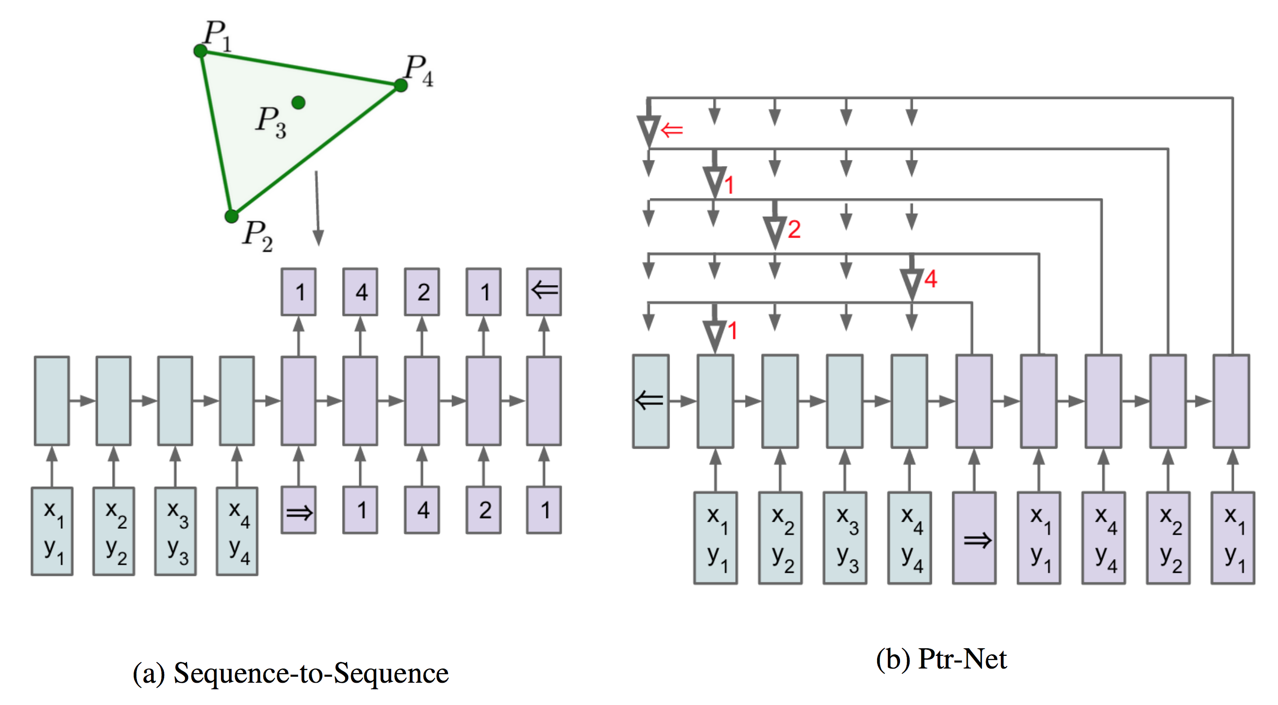
In traditional sequence-to-sequence RNN, output classes depend on
pre-defined size. For instance, a word generating RNN will utter one
word from vocabulary of \(|V|\) size at
each time step. However, there is large set of problems such as Convex
Hull, Delaunay Triangulation and TSP, where range of the each output is
not pre-defined, but of variable size, defined by the input. Pointer
Networks overcame the constraint by selecting \(i\) -th input with probability derived from
attention score.
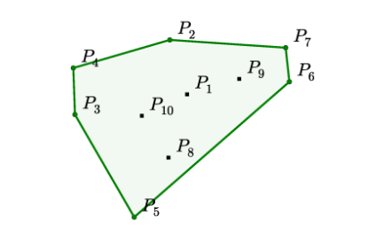
Convex Hull
In following example, 10 points are given, the output is a sequence
of points that bounds the set of all points. Each value in the output
sequence is a integer ranging from 1 to 10, in this case, which is the
value given by the concrete example. Generally, finding exact solution
has been proven to be equivelent to sort problem, and has time
complexity \(O(n*log(n))\).
TSP is almost identical to Convex Hull problem, though output
sequence is of fixed length. In previous epsiode, we reduced from \(O(n!)\) to \(O(n^2*2^n)\).
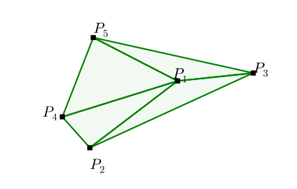
A Delaunay triangulation for a set of points in a plane is a
triangulation such that each circumcircle of every triangle is empty,
meaning no point from \(\mathcal{P}\)
in its interior. This kind of problem outputs a sequence of sets, and
each item in the set ranges from the input set \(\mathcal{P}\).
Suppose now n is fixed. given a training pair, \((\mathcal{P}, C^{\mathcal{P}})\), the
vanilla sequence-to-sequence model parameterized by \(\theta\) computes the conditional
probability.
\[
\begin{equation}
p\left(\mathcal{C}^{\mathcal{P}} | \mathcal{P} ;
\theta\right)=\prod_{i=1}^{m(\mathcal{P})} p\left(C_{i} | C_{1}, \ldots,
C_{i-1}, \mathcal{P} ; \theta\right)
\end{equation}
\] The parameters of the model are learnt by maximizing the
conditional probabilities for the training set, i.e. \[
\begin{equation}
\theta^{*}=\underset{\theta}{\arg \max } \sum_{\mathcal{P},
\mathcal{C}^{\mathcal{P}}} \log p\left(\mathcal{C}^{\mathcal{P}} |
\mathcal{P} ; \theta\right)
\end{equation}
\]
Content Based Input
Attention
When attention is applied to vanilla sequence-to-sequence model,
better result is obtained.
Let encoder and decoder states be $ (e_{1}, , e_{n}) $ and $ (d_{1},
, d_{m()}) $, respectively. At each output time \(i\), compute the attention vector \(d_i\) to be linear combination of $ (e_{1},
, e_{n}) $ with weights $ (a_{1}^{i}, , a_{n}^{i}) $ \[
d_{i} = \sum_{j=1}^{n} a_{j}^{i} e_{j}
\]
$ (a_{1}^{i}, , a_{n}^{i}) $ is softmax value of $ (u_{1}^{i}, ,
u_{n}^{i}) $ and \(u_{j}^{i}\) can be
considered as distance between \(d_{i}\) and \(e_{j}\). Notice that \(v\), \(W_1\), and \(W_2\) are learnable parameters of the
model.
Pointer Networks does not blend the encoder state \(e_j\) to propagate extra information to the
decoder, but instead, use \(u^i_j\) as
pointers to the input element.
In FloydHub Blog - Attention Mechanism , a clear and
detailed explanation of difference and similarity between the classic
first type of Attention, commonly referred to as Additive Attention by
Dzmitry Bahdanau and second classic type, known as
Multiplicative Attention and proposed by Thang Luong , is
discussed.
It's well known that in Luong Attention, three ways of alignment scoring
function is defined, or the distance between \(d_{i}\) and \(e_{j}\).
In episode 2, we have introduced TSP
dataset where each case is a line, of following form.
1
x0, y0, x1, y1, ... output 1 v1 v2 v3 ... 1
PyTorch Dataset
Each case is converted to (input, input_len, output_in, output_out,
output_len) of type nd.ndarray with appropriate padding and encapsulated
in a extended PyTorch Dataset.
{linenos
1 2 3 4 5 6 7 8 9 10 11 12
from torch.utils.data import Dataset
classTSPDataset(Dataset): "each data item of form (input, input_len, output_in, output_out, output_len)" data: List[Tuple[np.ndarray, np.ndarray, np.ndarray, np.ndarray, np.ndarray]] def__len__(self): returnlen(self.data)
Code in PyTorch seq-to-seq model typically utilizes
pack_padded_sequence and
pad_packed_sequence API to reduce computational cost. A
detailed explanation is given here
https://github.com/sgrvinod/a-PyTorch-Tutorial-to-Image-Captioning#decoder-1.
In last episode, we provided a top down recursive DP in Python 3 and
Java 8. Now we continue to improve and convert it to bottom up iterative
DP version. Below is a graph with 3 vertices, the top down recursive
calls are completely drawn.
Looking from bottom up, we could identify corresponding topological
computing order with ease. First, we compute all bit states with 3 ones,
then 2 ones, then 1 one.
Pseudo Java code below.
1 2 3 4 5 6 7 8 9 10 11 12 13 14 15 16
for (int bitset_num = N; bitset_num >=0; bitset_num++) { while(hasNextCombination(bitset_num)) { int state = nextCombination(bitset_num); // compute dp[state][v], v-th bit is set in state for (int v = 0; v < n; v++) { for (int u = 0; u < n; u++) { // for each u not reached by this state if (!include(state, u)) { dp[state][v] = min(dp[state][v], dp[new_state_include_u][u] + dist[v][u]); } } } } }
For example, dp[00010][1] is the min distance starting from vertex 0,
and just arriving at vertex 1: \(0 \rightarrow
1 \rightarrow ? \rightarrow ? \rightarrow ? \rightarrow 0\). In
order to find out total min distance, we need to enumerate all possible
u for first question mark. \[
(0 \rightarrow 1) +
\begin{align*}
\min \left\lbrace
\begin{array}{r@{}l}
2 \rightarrow ? \rightarrow ? \rightarrow 0 + dist(1,2)
\qquad\text{ new_state=[00110][2] } \qquad\\\\
3 \rightarrow ? \rightarrow ? \rightarrow 0 + dist(1,3)
\qquad\text{ new_state=[01010][3] } \qquad\\\\
4 \rightarrow ? \rightarrow ? \rightarrow 0 + dist(1,4)
\qquad\text{ new_state=[10010][4] } \qquad
\end{array}
\right.
\end{align*}
\]
Java Iterative DP Code
AC code in Python
3 and Java
8. Illustrate core Java code below.
publiclongsolve(){ int N = g.V_NUM; long[][] dp = newlong[1 << N][N]; // init dp[][] with MAX for (int i = 0; i < dp.length; i++) { Arrays.fill(dp[i], Integer.MAX_VALUE); } dp[(1 << N) - 1][0] = 0;
for (int state = (1 << N) - 2; state >= 0; state--) { for (int v = 0; v < N; v++) { for (int u = 0; u < N; u++) { if (((state >> u) & 1) == 0) { dp[state][v] = Math.min(dp[state][v], dp[state | 1 << u][u] + g.edges[v][u]); } } } } return dp[0][0] == Integer.MAX_VALUE ? -1 : dp[0][0]; }
In this way, runtime complexity can be spotted easily, three for
loops leading to O(\(2^n * n * n\)) =
O(\(2^n*n^2\) ).
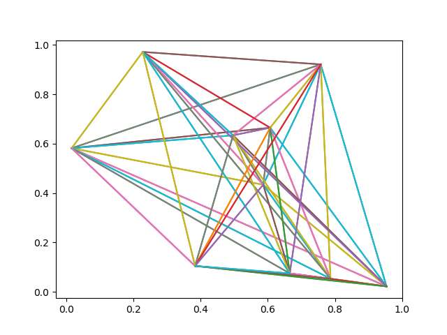
DP on Euclidean Dataset
So far, TSP DP has been crystal clear and we move forward to
introducing PTR_NET dataset on Google
Drive by Oriol Vinyals who is the author of Pointer Networks. Each line
in the dataset has the following pattern:
1
x0, y0, x1, y1, ... output 1 v1 v2 v3 ... 1
It first lists n points in (x, y) coordinate, followed by "output",
then followed by one of the minimal distance tours, starting and ending
with vertex 1 (indexed from 1 not 0).
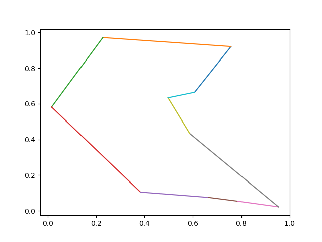
for i inrange(0, len(tour)-1): p1 = tour[i] - 1 p2 = tour[i + 1] - 1 plt.plot((x[p1],x[p2]),(y[p1],y[p2])) plt.show()
TSP Case Minimal Tour
Python Code Illustrated
Init Graph Edges
Based on previous top down version, several changes are made. First,
we need to have an edge between every 2 vertices and due to our matrix
representation of the directed edge, edges of 2 directions are
initialized.
{linenos
1 2 3 4 5 6 7 8
g: Graph = Graph(N) for v inrange(N): for u inrange(N): diff_x = coordinates[v][0] - coordinates[u][0] diff_y = coordinates[v][1] - coordinates[u][1] dist: float = math.sqrt(diff_x * diff_x + diff_y * diff_y) g.setDist(u, v, dist) g.setDist(v, u, dist)
Auxilliary Variable
to Track Tour Vertices
One major enhancement is to record the optimal tour during
enumerating. We introduce another variable parent[bitstate][v] to track
next vertex u, with shortest path.
{linenos
1
2
3
4
5
6
7
8
9
10
11
ret: float = FLOAT_INF u_min: int = -1 for u inrange(self.g.v_num): if (state & (1 << u)) == 0: s: float = self._recurse(u, state | 1 << u) if s + edges[v][u] < ret: ret = s + edges[v][u] u_min = u dp[state][v] = ret self.parent[state][v] = u_min
After minimal tour distance is found, one optimal tour is formed with
the help of parent variable.
{linenos
1 2 3 4 5 6 7 8 9
def_form_tour(self): self.tour = [0] bit = 0 v = 0 for _ inrange(self.g.v_num - 1): v = self.parent[bit][v] self.tour.append(v) bit = bit | (1 << v) self.tour.append(0)
Note that for each test case, only one tour is given after "output".
Our code may form a different tour but it has same distance as what the
dataset generates, which can be verified by following code snippet. See
full code on github.
Travelling
salesman problem (TSP) is a classic NP hard computer algorithmic
problem. In this series, we will first solve TSP problem in an exact
manner by ACing TSP on aizu with dynamic programming, and then move on
to train a Pointer Network with Pytorch to obtain an approximate
solution with deep learning and reinforcement learning technology.
Complete episodes are listed as follows:
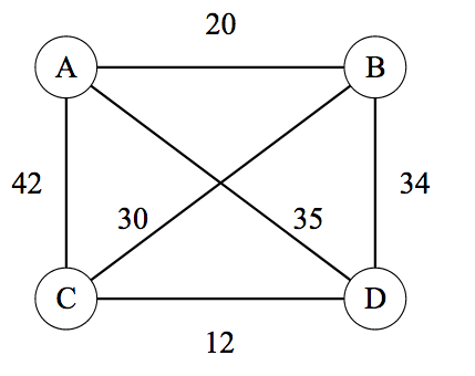
TSP can be modelled as a graph problem where both directed and
undirected graphs and both completely or partially connected graphs are
applicable. The following picture in Wikipedia
TSP is an undirected but complete TSP with four vertices, A, B, C,
D. TSP requries a tour with minimal total distance, starting from
arbitrarily picked vertex and ending with the same node while covering
all vertices exactly once. For example, \(A
\rightarrow B \rightarrow C \rightarrow D \rightarrow A\) and
\(A \rightarrow C \rightarrow B \rightarrow D
\rightarrow A\) are valid tours and among all tours there is only
one minimal distance value (though multiple tours with same minimum may
exist).
Wikipedia 4 Vertices Example
Despite different types of graphs, notice that we can always employ an
adjacency matrix to represent a graph. The above graph can thus be
represented by this matrix
Of course, typically, TSP problem takes the form of n cooridanates in
a plane, corresponding to complete and undirected graph, because in
plane every pair of vertices has one connected edge and the edge has
same distance in both directions.
AIZU TSP Online Judge
AIZU
has a TSP problem where a directed and incomplete graph with V vertices
and E directed edges is given, and the output expects minimal total
distance. For example below having 4 vertices and 6 edges.
This test case has minimal tour distance 16, with corresponding tour
being \(0\rightarrow1\rightarrow3\rightarrow2\rightarrow0\),
as shown in red edges. However, the AIZU problem may not have a valid
result because not every pair of vertices is guaranteed to be connected.
In that case, -1 is required, which can also be interpreted as
infinity.
Brute Force Solution
A naive way is to enumerate all possible routes starting from vertex
0 and keep minimal total distance ever generated. Python code below
illustrates a 4 point vertices graph.
{linenos
1
2
3
4
5
from itertools import permutations v = [1,2,3] p = permutations(v) for t inlist(p): print([0] + list(t) + [0])
This approach has a runtime
complexity of O(\(n!\)), which won't
pass AIZU.
Dynamic Programming
To AC AIZU TSP, we need to have acceleration of the factorial runtime
complexity by using bitmask dynamic programming. First, let us map
visited state to a binary value. In the 4 vertices case, it's "0110" if
node 2 and 1 already visited and ending at node 1. Besides, we need to
track current vertex to start from. So we extend dp from one dimension
to two dimensions \(dp[bitstate][v]\).
In the example, it's \(dp["0110"][1]\). The transition
formula is given by \[
dp[bitstate][v] = \min ( dp[bitstate \cup \{u\}][u] + dist(v,u) \mid u
\notin bitstate )
\]
The resulting time complexity is O(\(n^2*2^n\) ), since there are \(2^n * n\) total states and for each state
one more round loop is needed. Factorial and exponential functions are
significantly different.
\(n!\)
\(n^2*2^n\)
n=8
40320
16384
n=10
3628800
102400
n=12
479001600
589824
n=14
87178291200
3211264
Pause a second and think about why bitmask DP works here. Notice
there are lots of redundant sub calls, one of which is hightlighted in
red ellipse below.
In this episode, a straightforward top down memoization DP version is
given in Python 3 and Java 8. Benefit of top down DP approach is that we
don't need to consider topological ordering when permuting all states.
Notice that there is a trick in Java, where each element of dp is
initialized as Integer.MAX_VALUE, so that only one statement is needed
to update new dp value.
1
res = Math.min(res, s + g.edges[v][u]);
However, the code simplicity is at
cost of clarity and care should be taken when dealing with actual INF
(not reachable case). In python version, we could have used the same
trick, perhaps by intializing with a large long value representing INF.
But for clarity, we manually handle different cases in if-else
statements and mark intial value as -1 (INT_INF).
1 2 3 4 5 6 7
INT_INF = -1

if s != INT_INF and edges[v][u] != INT_INF:
    if ret == INT_INF:
        ret = s + edges[v][u]
    else:
        ret = min(ret, s + edges[v][u])
Below is complete AC code in Python 3 and Java 8. Also can be
downloaded on github.
publicGraph(int V_NUM){ this.V_NUM = V_NUM; this.edges = newint[V_NUM][V_NUM]; for (int i = 0; i < V_NUM; i++) { Arrays.fill(this.edges[i], Integer.MAX_VALUE); } } publicvoidsetDist(int src, int dest, int dist){ this.edges[src][dest] = dist; } } publicstaticclassTSP{ publicfinal Graph g; long[][] dp; publicTSP(Graph g){ this.g = g; } publiclongsolve(){ int N = g.V_NUM; dp = newlong[1 << N][N]; for (int i = 0; i < dp.length; i++) { Arrays.fill(dp[i], -1); } long ret = recurse(0, 0); return ret == Integer.MAX_VALUE ? -1 : ret; } privatelongrecurse(int state, int v){ int ALL = (1 << g.V_NUM) - 1; if (dp[state][v] >= 0) { return dp[state][v]; } if (state == ALL && v == 0) { dp[state][v] = 0; return0; } long res = Integer.MAX_VALUE; for (int u = 0; u < g.V_NUM; u++) { if ((state & (1 << u)) == 0) { long s = recurse(state | 1 << u, u); res = Math.min(res, s + g.edges[v][u]); } } dp[state][v] = res; return res; } } publicstaticvoidmain(String[] args){ Scanner in = new Scanner(System.in); int V = in.nextInt(); int E = in.nextInt(); Graph g = new Graph(V); while (E > 0) { int src = in.nextInt(); int dest = in.nextInt(); int dist = in.nextInt(); g.setDist(src, dest, dist); E--; } System.out.println(new TSP(g).solve()); } }
def__init__(self, v_num: int): self.v_num = v_num self.edges = [[INT_INF for c inrange(v_num)] for r inrange(v_num)] defsetDist(self, src: int, dest: int, dist: int): self.edges[src][dest] = dist
classTSPSolver: g: Graph dp: List[List[int]]
def__init__(self, g: Graph): self.g = g self.dp = [[Nonefor c inrange(g.v_num)] for r inrange(1 << g.v_num)] defsolve(self) -> int: return self._recurse(0, 0) def_recurse(self, v: int, state: int) -> int: """ :param v: :param state: :return: -1 means INF """ dp = self.dp edges = self.g.edges if dp[state][v] isnotNone: return dp[state][v] if (state == (1 << self.g.v_num) - 1) and (v == 0): dp[state][v] = 0 return dp[state][v] ret: int = INT_INF for u inrange(self.g.v_num): if (state & (1 << u)) == 0: s: int = self._recurse(u, state | 1 << u) if s != INT_INF and edges[v][u] != INT_INF: if ret == INT_INF: ret = s + edges[v][u] else: ret = min(ret, s + edges[v][u]) dp[state][v] = ret return ret