import numpy as np import torch import torch.nn as nn import torch.nn.functional as F
from torch_geometric.data import Data from torch_geometric.nn import GATConv from torch_geometric.datasets import Planetoid import torch_geometric.transforms as T
import matplotlib.pyplot as plt import networkx as nx
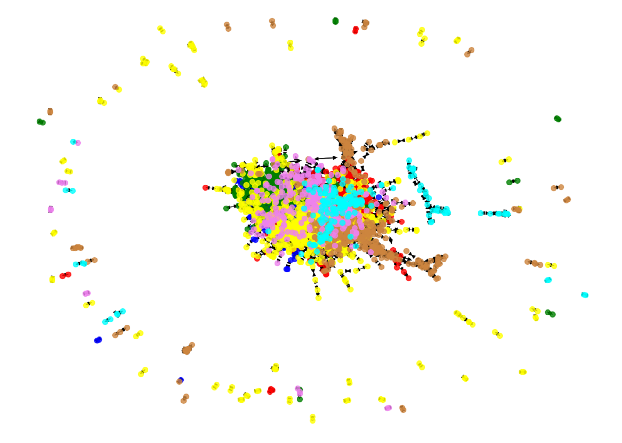
pos = nx.layout.spring_layout(cora)
我们首先来看一下 matplotlib 的渲染效果。
1 2 3 4 5 6 7 8 9 10 11
plt.figure(figsize=(16,12))
for i in np.arange(len(np.unique(node_classes))): node_list = node_label[node_classes == i] nx.draw_networkx_nodes(cora, pos, nodelist=list(node_list), node_size=50, node_color=node_color[i], alpha=0.8)
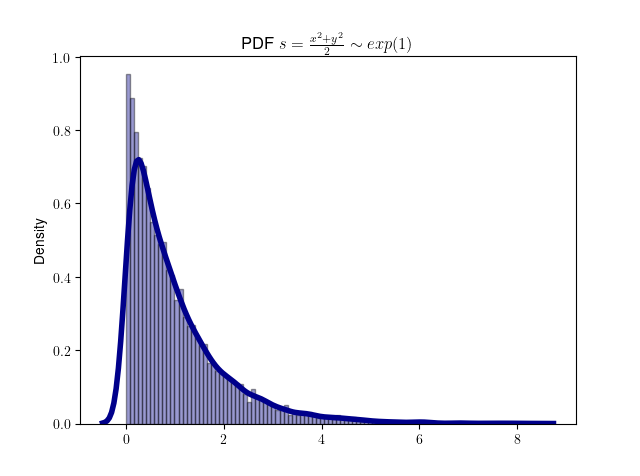
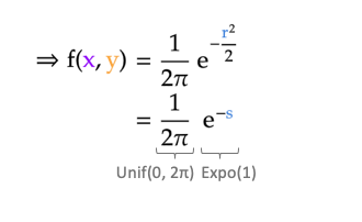
defnormal_box_muller(): import random from math import sqrt, log, pi, cos, sin u1 = random.random() u2 = random.random() r = sqrt(-2 * log(u1)) theta = 2 * pi * u2 z0 = r * cos(theta) z1 = r * sin(theta) return z0, z1
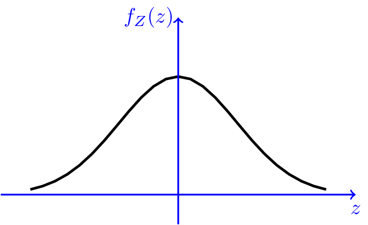
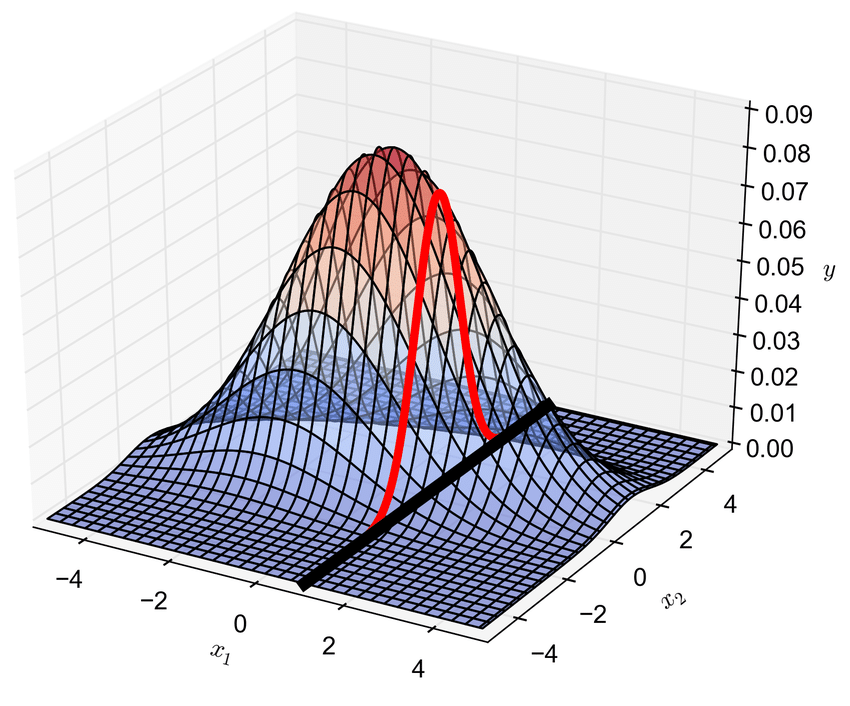
接下来,我们来看看 Box-Muller 法生成的二维标准正态分布动画吧
拒绝采样极坐标方法
Box-Muller 方法还有一种形式,称为极坐标形式,属于拒绝采样方法。
1. 生成独立的 u, v 和 s
分别生成 [0, 1] 均匀分布 u 和 v。令 \(s =
r^2 = u^2 + v^2\)。如果 s = 0或 s ≥ 1,则丢弃 u 和 v
,并尝试另一对 (u , v)。因为 u 和 v
是均匀分布的,并且因为只允许单位圆内的点,所以 s
的值也将均匀分布在开区间 (0, 1) 中。注意,这里的 s
的意义虽然也为半径,但不同于基本方法中的 s。这里 s 取值范围为
(0, 1) ,目的是通过 s 生成指数分布,而基本方法中的 s 取值范围为 [0,
+∞],表示二维正态分布 PDF 采样点的半径。复用符号 s
的原因是为了对应维基百科中关于基本方法和极坐标方法的数学描述。
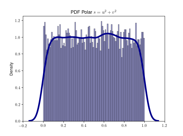
我们用代码来验证 s 服从 (0, 1) 范围上的均匀分布。
1 2 3 4 5 6 7 8 9 10 11 12 13 14
defgen_polar_s(): import random whileTrue: u = random.uniform(-1, 1) v = random.uniform(-1, 1) s = u * u + v * v if s >= 1.0or s == 0.0: continue return s
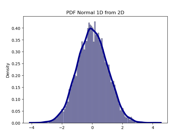
defplot_polar_s(): s = [gen_polar_s() for _ inrange(10000) ] plot_dist_1d(s, title='PDF Polar $s = u^2 + v^2$')
defnormal_box_muller_polar(): import random from math import sqrt, log whileTrue: u = random.uniform(-1, 1) v = random.uniform(-1, 1) s = u * u + v * v if s >= 1.0or s == 0.0: continue z0 = u * sqrt(-2 * log(s) / s) z1 = v * sqrt(-2 * log(s) / s) return z0, z1
Lecture
1 - Introduction to Unleashing Novel Data at Scale
Why data accessibility is so central to the advancement of knowledge
in economics (with some historical background)
An overview of the data curation pipeline
Step 1: Detect document layouts
Step 2: OCR
Step 3: Post-processing and database assembly
Step 4: Convert information into computable format
Why is the material covered in this course useful to social
scientists?
Why there won’t be an app/commercial product capable of end-to-end
processing of social science documents anytime soon
Why manual data entry often falls short
Why our problems differ from those that are the central focus of
computer science and the digital humanities
At its core, deep learning is an optimization problem, which
economists are well-trained to understand. It would be really
unfortunate if we did not take full advantage of the very powerful
methods that deep learning offers, which we are well poised to
utilize
Lecture 2 - Why Deep
Learning?
This post compares rule-based and deep learning-based approaches to
data curation. It discusses their requirements and why rule-based
approaches often (but not always) produce disappointing results when
applied to social science data.
An overview of the syllabus (ultimately, the course had a few
deviations from the original syllabus, based on student interests; final
syllabus posted in the course section of this website)
There are two distinct approaches to automated data curation
Tell the computer how to process the data by defining a set of
rules
Let the computer learn how to process the data from empirical
examples, using deep learning
Overview of rules, how they are used to process image scans and
text, why they often fail, and why they sometimes succeed
Deep learning, how it contrasts with rule-based approaches, and its
requirements
Does the noise from rule-based approaches really matter?
Lecture 4 -
Convolutional Neural Networks
A brief overview of convolutions
Benchmark datasets for image classification (following the ConvNent
literature requires familiarity with the benchmarks)
Image classification with a linear classifier (and its
shortcomings)
CNN architectures
AlexNet
VGG
GoogLeNet
ResNet
ResNext
Lecture 5
- Image Classification; Training Neural Nets
This post covers two topics: using CNNs for image classification (a
very useful task) and training neural networks in practice. Much of the
information about training neural nets is essential to implementing deep
learning-based approaches, whether with CNNs or with some other
architecture.
Image Classification
Loss functions for classification
SVM
Softmax
Deep document classification
Training Neural Nets
Activation functions
Data pre-processing
Initialization
Optimization
Regularization
Batch normalization
Dropout
Data augmentation
Transfer learning
Setting hyperparameters
Monitoring the learning process
Lecture
6 - Other Computer Vision Problems (Including Object Detection)
This post covers object detection as well as the related problems of
semantic segmentation, localization, and instance segmentation. Object
detection is core to document image analysis, as it is used to determine
the coordinates and classes of different document layout regions. The
other problems covered are closely related.
Semantic segmentation
Localization
Object detection
Region CNNs
Fast R-CNN
Faster R-CNN
Mask R-CNN
Features pyramids
Instance segmentation
Other frameworks (YOLO)
Lecture 7 - Object
Detection in Practice
Selecting an object detection model
Overview of Detectron2
How-to in D2
Lecture 8 -
Labeling and Deep Visualization
Labeling
Active learning for layout annotation
Labeling hacks
Deep visualization
Basic visualization approaches
Gradient based ascent
Deep Dream
Lecture 9 -
Generative Adversarial Networks
Overview: supervised and unsupervised learning; generative
models
Generative adversarial networks
CycleGAN
Lecture 10 - OCR
Architecture
Overview of the OCR problem
Recurrent neural networks
LSTMs
Connectionist temporal classification
Putting it together
Lecture 11 -
OCR and Post-Processing in Practice
This post discusses OCR, both off-the-shelf and how to implement a
customized OCR model. It discusses how Layout Parser can be used for
end-to-end document image analysis, and provides concrete examples of
creating variable domains during post-processing. It also provides an
overview of the second half of the knowledge base, which covers NLP.
Off-the-shelf OCR
Designing customized OCR
Putting it altogether (and Layout Parser)
Creating variable domains
An overview of the second half of the course (NLP)
Lecture 12 - Models of Words
Traditional models of words
Word2Vec
GloVe
Evaluation
Interpreting word vectors
Problems with word vectors
Lecture
13 - Language Modeling and Other Topics in NLP
This post provides an introduction to language modeling, as well as
several other important topics: dependency parsing, named entity
recognition (NER), and labeling for NLP. Due to time constraints, the
course is able to provide only a very brief introduction to topics like
dependency parsing and NER, which have traditionally been quite central
questions in NLP research.
Language Modeling
Count based models
Bag of words
RNN (review)
LSTM (review)
Dependency parsing
Named entity recognition
Labeling for NLP
Lecture 14 -
Seq2Seq and Machine Translation
Machine translation has pioneered some of the most productive
innovations in neural-based NLP and hence is useful to study even for
those who care little about machine translation per se. We will focus in
particular on seq2seq and attention.
Statistical machine translation
Neural machine translation
Lecture 15 - Attention
is All You Need
This post introduces the Transformer, a seq2seq model based entirely
on attention that has transformed NLP. Given the importance of this
paper, there are a bunch of very well-done web resources about it, cited
in the lecture and below, that I recommend checking out directly (there
are others who have much more of a comparative advantage in presenting
seminal NLP papers than I do!).
A recap of attention
The Transformer
The encoder
Encoder self-attention
Positional embeddings
Add and normalize
The decoder
Encoder-decoder attention
Decoder self-attention
Linear and softmax layers
Training
Lecture 16 -
Transformer-Based Language Models
This post provides an overview of various Transformer-based language
models, discussing their architectures and which are best-suited for
different contexts.
Overview
Contextualized word embeddings
Models
GPT
BERT
RoBERTa
DistilBERT
ALBERT
T5
GPT2/GPT3
Transformers XL
XLNet
Longformer
BigBird
Recap and what to use
Lecture
17 - Understanding Transformers, Visualization, and Sentiment
Analysis
This post covers a variety of topics around Transformer-based
language models: understanding how Transformer attention works,
understanding what information is contained in their embeddings,
visualizing embeddings, and using Transformer-based models to conduct
sentiment analysis.
What do Transformer-based models attend to?
What’s in an embedding?
Visualizing embeddings
Sentiment analysis
Lecture 18 - NLP with Noisy
Text
The Canonical Deep NLP Training Corpus
A definition of noise
The problem with noise
Approaches for denoising
Lecture 19 -
Retrieval and Question Answering
Reading comprehension
Open-domain question answering
Lecture 20
- Zero-Shot and Few-Shot Learning in NLP
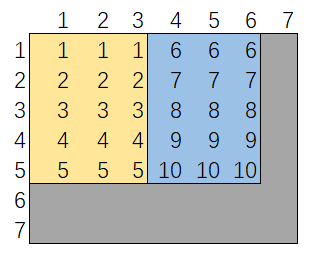
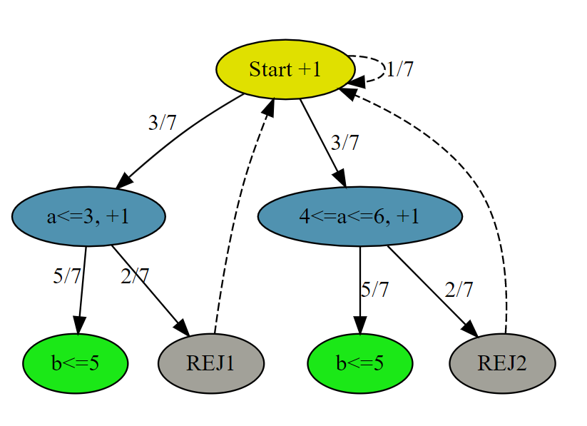
# AC # Runtime: 408 ms, faster than 23.80% of Python3 online submissions for Implement Rand10() Using Rand7(). # Memory Usage: 16.7 MB, less than 90.76% of Python3 online submissions for Implement Rand10() Using Rand7(). classSolution: defrand10(self): whileTrue: a = rand7() if a <= 3: b = rand7() if b <= 5: return b elif a <= 6: b = rand7() if b <= 5: return b + 5
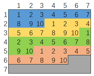
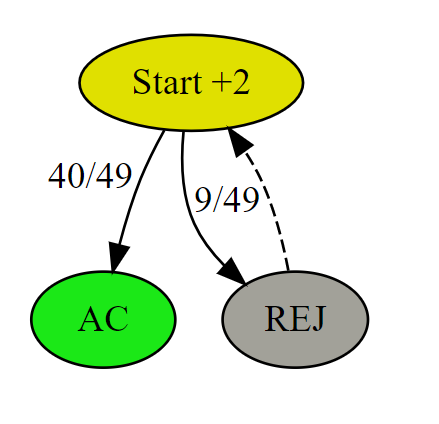
# AC # Runtime: 376 ms, faster than 54.71% of Python3 online submissions for Implement Rand10() Using Rand7(). # Memory Usage: 16.9 MB, less than 38.54% of Python3 online submissions for Implement Rand10() Using Rand7(). classSolution: defrand10(self): whileTrue: a, b = rand7(), rand7() num = (a - 1) * 7 + b if num <= 40: return num % 10 + 1
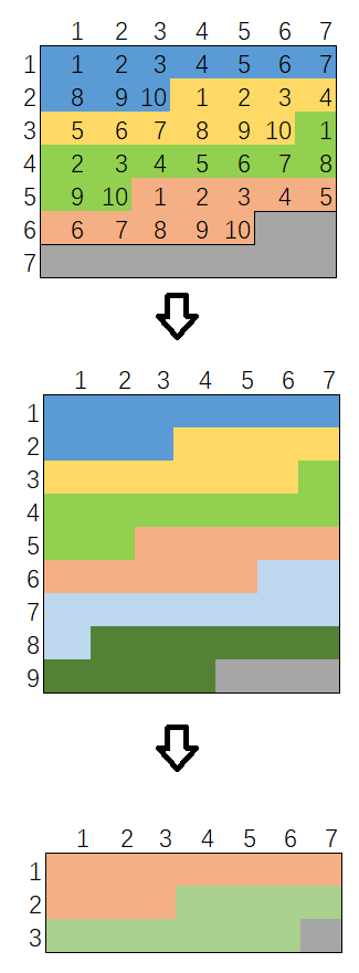
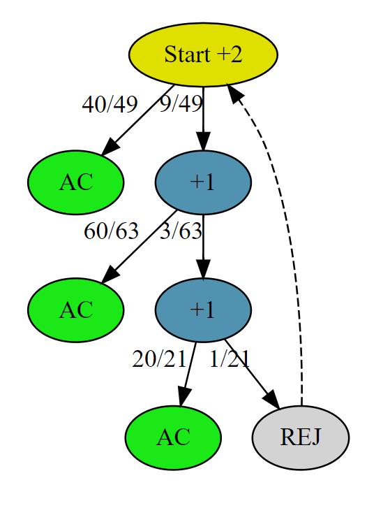
# AC # Runtime: 344 ms, faster than 92.72% of Python3 online submissions for Implement Rand10() Using Rand7(). # Memory Usage: 16.7 MB, less than 90.76% of Python3 online submissions for Implement Rand10() Using Rand7(). classSolution: defrand10(self): whileTrue: a, b = rand7(), rand7() num = (a - 1) * 7 + b if num <= 40: return num % 10 + 1 a = num - 40 b = rand7() num = (a - 1) * 7 + b if num <= 60: return num % 10 + 1 a = num - 60 b = rand7() num = (a - 1) * 7 + b if num <= 20: return num % 10 + 1
# The rand7() API is already defined for you. rand7_c = 0 rand10_c = 0
defrand7(): global rand7_c rand7_c += 1 import random return random.randint(1, 7) defrand10(): global rand10_c rand10_c += 1 whileTrue: a, b = rand7(), rand7() num = (a - 1) * 7 + b if num <= 40: return num % 10 + 1 a = num - 40# [1, 9] b = rand7() num = (a - 1) * 7 + b # [1, 63] if num <= 60: return num % 10 + 1 a = num - 60# [1, 3] b = rand7() num = (a - 1) * 7 + b # [1, 21] if num <= 20: return num % 10 + 1
if __name__ == '__main__': whileTrue: rand10() print(f'{rand10_c}{round(rand7_c/rand10_c, 2)}')
classActions(Enum): """ Different settings for the action space of the environment """ ALL = 0#: MultiBinary action space with no filtered actions FILTERED = 1#: MultiBinary action space with invalid or not allowed actions filtered out DISCRETE = 2#: Discrete action space for filtered actions MULTI_DISCRETE = 3#: MultiDiscete action space for filtered actions
from gym.spaces import * space = Dict({'position':Discrete(2), 'velocity':Discrete(3)}) print(space.sample())
输出是
1
OrderedDict([('position', 1), ('velocity', 1)])
NES 1942 动作空间配置
了解了 gym/retro 的动作空间,我们来看看1942的默认动作空间
1 2
env = retro.make(game='1942-Nes') print("The size of action is: ", env.action_space.shape)
1
The size of action is: (9,)
表示有9个 Discrete 动作,包括 start, select这些控制键。
从训练1942角度来说,我们希望指定最少的有效动作取得最好的成绩。根据经验,我们知道这个游戏最重要的键是4个方向加上
fire
键。限定游戏动作空间,官方的做法是在创建游戏环境时,指定预先生成的动作输入配置文件。但是这个方式相对麻烦,我们采用了直接指定按键的二进制表示来达到同样的目的,此时,需要设置
use_restricted_actions=retro.Actions.FILTERED。
for _ inrange(self.ppo_epoch): for state, action, old_log_probs, return_, advantage in sample_batch(): dist = self.actor_net(state) value = self.critic_net(state)
# Minimize the loss self.actor_optimizer.zero_grad() self.critic_optimizer.zero_grad() loss.backward() self.actor_optimizer.step() self.critic_optimizer.step()
最直接的方式是暴力枚举出所有分组的可能。因为 2N
个人平均分成两组,总数为 \({2n \choose
n}\),是 n 的指数级数量。在文章24
点游戏算法题的 Python 函数式实现: 学用itertools,yield,yield from
巧刷题,我们展示如何调用 Python 的
itertools包,这里,我们也用同样的方式产生 [0, 2N]
的所有集合大小为N的可能(保存在left_set_list中),再遍历找到最小值即可。当然,这种解法会TLE,只是举个例子来体会一下暴力做法。
{linenos
1 2 3 4 5 6 7 8 9 10 11 12 13 14 15 16 17 18
import math from typing importList
classSolution: deftwoCitySchedCost(self, costs: List[List[int]]) -> int: L = range(len(costs)) from itertools import combinations left_set_list = [set(c) for c in combinations(list(L), len(L)//2)]
min_total = math.inf for left_set in left_set_list: cost = 0 for i in L: is_left = 1if i in left_set else0 cost += costs[i][is_left] min_total = min(min_total, cost)
return min_total
O(N) AC解法
对于组合优化问题来说,例如TSP问题(解法链接 TSP问题从DP算法到深度学习1:递归DP方法
AC AIZU TSP问题),一般都是
NP-Hard问题,意味着没有多项次复杂度的解法。但是这个问题比较特殊,它增加了一个特定条件:去城市A和城市B的人数相同,也就是我们已经知道两个分组的数量是一样的。我们仔细思考一下这个意味着什么?考虑只有四个人的小规模情况,如果让你来手动规划,你一定不会穷举出所有两两分组的可能,而是比较人与人相对的两个城市的cost差。举个例子,有如下四个人的costs
# AC # Runtime: 36 ms, faster than 87.77% of Python3 online submissions # Memory Usage: 14.5 MB, less than 14.84% of Python3 online from typing importList
classSolution: deftwoCitySchedCost(self, costs: List[List[int]]) -> int: L = range(len(costs)) cost_diff_lst = [(i, costs[i][0] - costs[i][1]) for i in L] cost_diff_lst.sort(key=lambda x: x[1])
total_cost = 0 for c, (idx, _) inenumerate(cost_diff_lst): is_left = 0if c < len(L) // 2else1 total_cost += costs[idx][is_left]
model = cp_model.CpModel() x = [] total_cost = model.NewIntVar(0, 10000, 'total_cost') for i in I: t = [] for j inrange(2): t.append(model.NewBoolVar('x[%i,%i]' % (i, j))) x.append(t)
# Constraints # Each person must be assigned to at exact one city [model.Add(sum(x[i][j] for j inrange(2)) == 1) for i in I] # equal number of person assigned to two cities model.Add(sum(x[i][0] for i in I) == (len(I) // 2))
# Total cost model.Add(total_cost == sum(x[i][0] * costs[i][0] + x[i][1] * costs[i][1] for i in I)) model.Minimize(total_cost)
solver = cp_model.CpSolver() status = solver.Solve(model)
if status == cp_model.OPTIMAL: print('Total min cost = %i' % solver.ObjectiveValue()) print() for i in I: for j inrange(2): if solver.Value(x[i][j]) == 1: print('People ', i, ' assigned to city ', j, ' Cost = ', costs[i][j])
items=[i for i in I] city_a = pulp.LpVariable.dicts('left', items, 0, 1, pulp.LpBinary) city_b = pulp.LpVariable.dicts('right', items, 0, 1, pulp.LpBinary)
m = pulp.LpProblem("Two Cities", pulp.LpMinimize)
m += pulp.lpSum((costs[i][0] * city_a[i] + costs[i][1] * city_b[i]) for i in items)
# Constraints # Each person must be assigned to at exact one city for i in I: m += pulp.lpSum([city_a[i] + city_b[i]]) == 1 # create a binary variable to state that a table setting is used m += pulp.lpSum(city_a[i] for i in I) == (len(I) // 2)
m.solve()
total = 0 for i in I: if city_a[i].value() == 1.0: total += costs[i][0] else: total += costs[i][1]