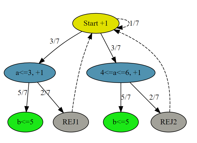
# AC # Runtime: 408 ms, faster than 23.80% of Python3 online submissions for Implement Rand10() Using Rand7(). # Memory Usage: 16.7 MB, less than 90.76% of Python3 online submissions for Implement Rand10() Using Rand7(). classSolution: defrand10(self): whileTrue: a = rand7() if a <= 3: b = rand7() if b <= 5: return b elif a <= 6: b = rand7() if b <= 5: return b + 5
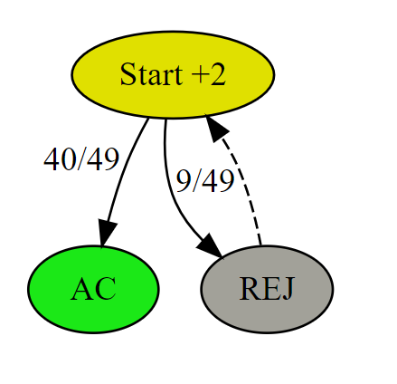
# AC # Runtime: 376 ms, faster than 54.71% of Python3 online submissions for Implement Rand10() Using Rand7(). # Memory Usage: 16.9 MB, less than 38.54% of Python3 online submissions for Implement Rand10() Using Rand7(). classSolution: defrand10(self): whileTrue: a, b = rand7(), rand7() num = (a - 1) * 7 + b if num <= 40: return num % 10 + 1
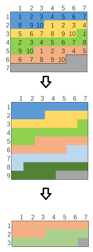
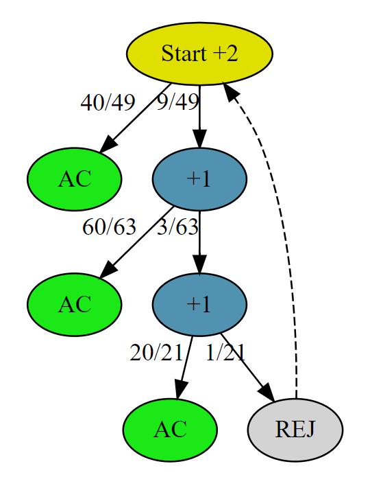
# AC # Runtime: 344 ms, faster than 92.72% of Python3 online submissions for Implement Rand10() Using Rand7(). # Memory Usage: 16.7 MB, less than 90.76% of Python3 online submissions for Implement Rand10() Using Rand7(). classSolution: defrand10(self): whileTrue: a, b = rand7(), rand7() num = (a - 1) * 7 + b if num <= 40: return num % 10 + 1 a = num - 40 b = rand7() num = (a - 1) * 7 + b if num <= 60: return num % 10 + 1 a = num - 60 b = rand7() num = (a - 1) * 7 + b if num <= 20: return num % 10 + 1
# The rand7() API is already defined for you. rand7_c = 0 rand10_c = 0
defrand7(): global rand7_c rand7_c += 1 import random return random.randint(1, 7) defrand10(): global rand10_c rand10_c += 1 whileTrue: a, b = rand7(), rand7() num = (a - 1) * 7 + b if num <= 40: return num % 10 + 1 a = num - 40# [1, 9] b = rand7() num = (a - 1) * 7 + b # [1, 63] if num <= 60: return num % 10 + 1 a = num - 60# [1, 3] b = rand7() num = (a - 1) * 7 + b # [1, 21] if num <= 20: return num % 10 + 1
if __name__ == '__main__': whileTrue: rand10() print(f'{rand10_c}{round(rand7_c/rand10_c, 2)}')
最直接的方式是暴力枚举出所有分组的可能。因为 2N
个人平均分成两组,总数为 \({2n \choose
n}\),是 n 的指数级数量。在文章24
点游戏算法题的 Python 函数式实现: 学用itertools,yield,yield from
巧刷题,我们展示如何调用 Python 的
itertools包,这里,我们也用同样的方式产生 [0, 2N]
的所有集合大小为N的可能(保存在left_set_list中),再遍历找到最小值即可。当然,这种解法会TLE,只是举个例子来体会一下暴力做法。
{linenos
1 2 3 4 5 6 7 8 9 10 11 12 13 14 15 16 17 18
import math from typing importList
classSolution: deftwoCitySchedCost(self, costs: List[List[int]]) -> int: L = range(len(costs)) from itertools import combinations left_set_list = [set(c) for c in combinations(list(L), len(L)//2)]
min_total = math.inf for left_set in left_set_list: cost = 0 for i in L: is_left = 1if i in left_set else0 cost += costs[i][is_left] min_total = min(min_total, cost)
return min_total
O(N) AC解法
对于组合优化问题来说,例如TSP问题(解法链接 TSP问题从DP算法到深度学习1:递归DP方法
AC AIZU TSP问题),一般都是
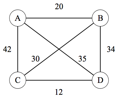
NP-Hard问题,意味着没有多项次复杂度的解法。但是这个问题比较特殊,它增加了一个特定条件:去城市A和城市B的人数相同,也就是我们已经知道两个分组的数量是一样的。我们仔细思考一下这个意味着什么?考虑只有四个人的小规模情况,如果让你来手动规划,你一定不会穷举出所有两两分组的可能,而是比较人与人相对的两个城市的cost差。举个例子,有如下四个人的costs
# AC # Runtime: 36 ms, faster than 87.77% of Python3 online submissions # Memory Usage: 14.5 MB, less than 14.84% of Python3 online from typing importList
classSolution: deftwoCitySchedCost(self, costs: List[List[int]]) -> int: L = range(len(costs)) cost_diff_lst = [(i, costs[i][0] - costs[i][1]) for i in L] cost_diff_lst.sort(key=lambda x: x[1])
total_cost = 0 for c, (idx, _) inenumerate(cost_diff_lst): is_left = 0if c < len(L) // 2else1 total_cost += costs[idx][is_left]
model = cp_model.CpModel() x = [] total_cost = model.NewIntVar(0, 10000, 'total_cost') for i in I: t = [] for j inrange(2): t.append(model.NewBoolVar('x[%i,%i]' % (i, j))) x.append(t)
# Constraints # Each person must be assigned to at exact one city [model.Add(sum(x[i][j] for j inrange(2)) == 1) for i in I] # equal number of person assigned to two cities model.Add(sum(x[i][0] for i in I) == (len(I) // 2))
# Total cost model.Add(total_cost == sum(x[i][0] * costs[i][0] + x[i][1] * costs[i][1] for i in I)) model.Minimize(total_cost)
solver = cp_model.CpSolver() status = solver.Solve(model)
if status == cp_model.OPTIMAL: print('Total min cost = %i' % solver.ObjectiveValue()) print() for i in I: for j inrange(2): if solver.Value(x[i][j]) == 1: print('People ', i, ' assigned to city ', j, ' Cost = ', costs[i][j])
items=[i for i in I] city_a = pulp.LpVariable.dicts('left', items, 0, 1, pulp.LpBinary) city_b = pulp.LpVariable.dicts('right', items, 0, 1, pulp.LpBinary)
m = pulp.LpProblem("Two Cities", pulp.LpMinimize)
m += pulp.lpSum((costs[i][0] * city_a[i] + costs[i][1] * city_b[i]) for i in items)
# Constraints # Each person must be assigned to at exact one city for i in I: m += pulp.lpSum([city_a[i] + city_b[i]]) == 1 # create a binary variable to state that a table setting is used m += pulp.lpSum(city_a[i] for i in I) == (len(I) // 2)
m.solve()
total = 0 for i in I: if city_a[i].value() == 1.0: total += costs[i][0] else: total += costs[i][1]
for v inrange(N): next_q.put(PQItem(initial[v], str(v)))
for l inrange(1, L): current_q = next_q next_q = PriorityQueue() k = K whilenot current_q.empty() and k > 0: item = current_q.get() prob, route, prev_v = item.prob, item.route, item.last_v k -= 1 for v inrange(N): nextItem = PQItem(prob * transition[prev_v][v], route + str(v)) next_q.put(nextItem)
for (int bitset_num = N; bitset_num >=0; bitset_num++) { while(hasNextCombination(bitset_num)) { int state = nextCombination(bitset_num); // compute dp[state][v], v-th bit is set in state for (int v = 0; v < n; v++) { for (int u = 0; u < n; u++) { // for each u not reached by this state if (!include(state, u)) { dp[state][v] = min(dp[state][v], dp[new_state_include_u][u] + dist[v][u]); } } } } }
ret: float = FLOAT_INF u_min: int = -1 for u inrange(self.g.v_num): if (state & (1 << u)) == 0: s: float = self._recurse(u, state | 1 << u) if s + edges[v][u] < ret: ret = s + edges[v][u] u_min = u dp[state][v] = ret self.parent[state][v] = u_min
当最终最短行程确定后,根据parent的信息可以按图索骥找到完整的行程顶点信息。
{linenos
1 2 3 4 5 6 7 8 9
def_form_tour(self): self.tour = [0] bit = 0 v = 0 for _ inrange(self.g.v_num - 1): v = self.parent[bit][v] self.tour.append(v) bit = bit | (1 << v) self.tour.append(0)
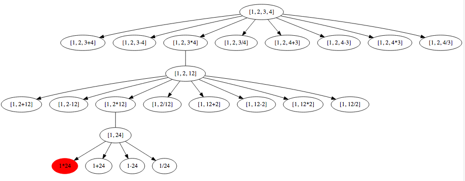
Leetcode 679 24 Game
(Hard) > You have 4 cards each containing a number from 1 to 9.
You need to judge whether they could operated through *, /, +, -, (, )
to get the value of 24.
# AC # Runtime: 36 ms, faster than 91.78% of Python3 online submissions for Permutations. # Memory Usage: 13.9 MB, less than 66.52% of Python3 online submissions for Permutations.
from itertools import permutations from typing importList
classSolution: defpermute(self, nums: List[int]) -> List[List[int]]: return [p for p in permutations(nums)]
# AC # Runtime: 84 ms, faster than 95.43% of Python3 online submissions for Combinations. # Memory Usage: 15.2 MB, less than 68.98% of Python3 online submissions for Combinations. from itertools import combinations from typing importList
classSolution: defcombine(self, n: int, k: int) -> List[List[int]]: return [c for c in combinations(list(range(1, n + 1)), k)]
itertools.product
当有多维度的对象需要迭代笛卡尔积时,可以用 product(iter1, iter2,
...)来生成generator,等价于多重 for 循环。
1 2
[lst for lst in product([1, 2, 3], ['a', 'b'])] [(i, s) for i in [1, 2, 3] for s in ['a', 'b']]
Given a string containing digits from 2-9 inclusive, return all
possible letter combinations that the number could represent. A mapping
of digit to letters (just like on the telephone buttons) is given below.
Note that 1 does not map to any letters.
# AC # Runtime: 24 ms, faster than 94.50% of Python3 online submissions for Letter Combinations of a Phone Number. # Memory Usage: 13.7 MB, less than 83.64% of Python3 online submissions for Letter Combinations of a Phone Number.
from itertools import product from typing importList
classSolution: defletterCombinations(self, digits: str) -> List[str]: if digits == "": return [] mapping = {'2':'abc', '3':'def', '4':'ghi', '5':'jkl', '6':'mno', '7':'pqrs', '8':'tuv', '9':'wxyz'} iter_dims = [mapping[i] for i in digits]
result = [] for lst in product(*iter_dims): result.append(''.join(lst))
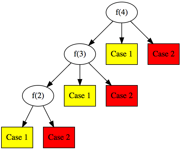
The Fibonacci numbers, commonly denoted F(n) form a sequence, called
the Fibonacci sequence, such that each number is the sum of the two
preceding ones, starting from 0 and 1. That is, F(0) = 0, F(1) = 1 F(N)
= F(N - 1) + F(N - 2), for N > 1. Given N, calculate F(N).
# AC # Runtime: 28 ms, faster than 85.56% of Python3 online submissions for Fibonacci Number. # Memory Usage: 13.8 MB, less than 58.41% of Python3 online submissions for Fibonacci Number.
classSolution: deffib(self, N: int) -> int: if N <= 1: return N i = 2 for fib in self.fib_next(): if i == N: return fib i += 1 deffib_next(self): f_last2, f_last = 0, 1 whileTrue: f = f_last2 + f_last f_last2, f_last = f_last, f yield f
yield from 示例
上述yield用法之后,再来演示 yield from 的用法。Yield from 始于Python
3.3,用于嵌套generator时的控制转移,一种典型的用法是有多个generator嵌套时,外层的outer_generator
用 yield from 这种方式等价代替如下代码。
1 2 3
defouter_generator(): for i in inner_generator(): yield i
# AC # Runtime: 48 ms, faster than 90.31% of Python3 online submissions for Kth Smallest Element in a BST. # Memory Usage: 17.9 MB, less than 14.91% of Python3 online submissions for Kth Smallest Element in a BST.
classSolution: defkthSmallest(self, root: TreeNode, k: int) -> int: defordered_iter(node): if node: for sub_node in ordered_iter(node.left): yield sub_node yield node for sub_node in ordered_iter(node.right): yield sub_node
for node in ordered_iter(root): k -= 1 if k == 0: return node.val
等价于如下 yield from 版本:
{linenos
1 2 3 4 5 6 7 8 9 10 11 12 13 14 15 16
# AC # Runtime: 56 ms, faster than 63.74% of Python3 online submissions for Kth Smallest Element in a BST. # Memory Usage: 17.7 MB, less than 73.33% of Python3 online submissions for Kth Smallest Element in a BST.
# AC # Runtime: 112 ms, faster than 57.59% of Python3 online submissions for 24 Game. # Memory Usage: 13.7 MB, less than 85.60% of Python3 online submissions for 24 Game.
import math from itertools import permutations, product from typing importList
defjudgePoint24(self, nums: List[int]) -> bool: mul = lambda x, y: x * y plus = lambda x, y: x + y div = lambda x, y: x / y if y != 0else math.inf minus = lambda x, y: x - y
op_lst = [plus, minus, mul, div]
for ops in product(op_lst, repeat=3): for val in permutations(nums): for v in self.iter_trees(ops[0], ops[1], ops[2], val[0], val[1], val[2], val[3]): ifabs(v - 24) < 0.0001: returnTrue returnFalse
# AC # Runtime: 116 ms, faster than 56.23% of Python3 online submissions for 24 Game. # Memory Usage: 13.9 MB, less than 44.89% of Python3 online submissions for 24 Game.
import math from itertools import combinations, product, permutations from typing importList
classSolution:
defjudgePoint24(self, nums: List[int]) -> bool: mul = lambda x, y: x * y plus = lambda x, y: x + y div = lambda x, y: x / y if y != 0else math.inf minus = lambda x, y: x - y
op_lst = [plus, minus, mul, div]
defrecurse(lst: List[int]): iflen(lst) == 2: for op, values in product(op_lst, permutations(lst)): yield op(values[0], values[1]) else: # choose 2 indices from lst of length n for choosen_idx_lst in combinations(list(range(len(lst))), 2): # remaining indices not choosen (of length n-2) idx_remaining_set = set(list(range(len(lst)))) - set(choosen_idx_lst)
# remaining values not choosen (of length n-2) value_remaining_lst = list(map(lambda x: lst[x], idx_remaining_set)) for op, idx_lst in product(op_lst, permutations(choosen_idx_lst)): # 2 choosen values are lst[idx_lst[0]], lst[idx_lst[1] value_remaining_lst.append(op(lst[idx_lst[0]], lst[idx_lst[1]])) yieldfrom recurse(value_remaining_lst) value_remaining_lst = value_remaining_lst[:-1]
for v in recurse(nums): ifabs(v - 24) < 0.0001: returnTrue
旅行商问题(TSP)是计算机算法中经典的NP
hard 问题。 在本系列文章中,我们将首先使用动态规划 AC
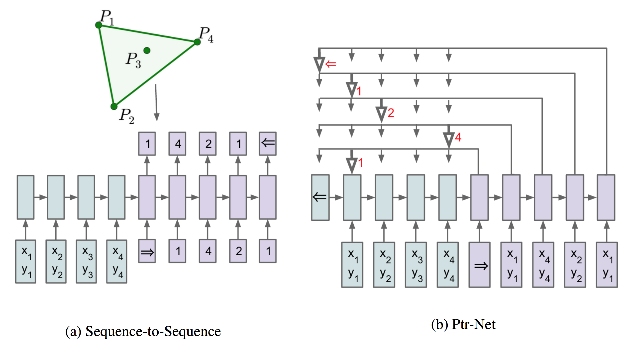
aizu中的TSP问题,然后再利用深度学习求大规模下的近似解。深度学习应用解决问题时先以PyTorch实现监督学习算法
Pointer Network,进而结合强化学习来无监督学习,提高数据使用效率。
本系列完整列表如下:
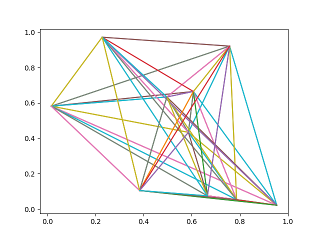
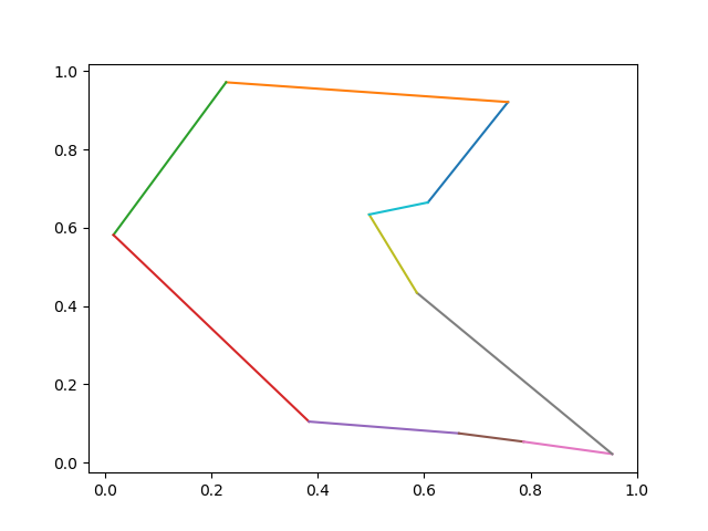
TSP可以用图模型来表达,无论有向图或无向图,无论全连通图或者部分连通的图都可以作为TSP问题。
Wikipedia
TSP
中举了一个无向全连通的TSP例子。如下图所示,四个顶点A,B,C,D构成无向全连通图。TSP问题要求在所有遍历所有点后返回初始点的回路中找到最短的回路。例如,\(A \rightarrow B \rightarrow C \rightarrow D
\rightarrow A\) 和 \(A \rightarrow C
\rightarrow B \rightarrow D \rightarrow A\)
都是有效的回路,但是TSP需要返回这些回路中的最短回路(注意,最短回路可能会有多条)。
publicGraph(int V_NUM){ this.V_NUM = V_NUM; this.edges = newint[V_NUM][V_NUM]; for (int i = 0; i < V_NUM; i++) { Arrays.fill(this.edges[i], Integer.MAX_VALUE); } } publicvoidsetDist(int src, int dest, int dist){ this.edges[src][dest] = dist; } } publicstaticclassTSP{ publicfinal Graph g; long[][] dp; publicTSP(Graph g){ this.g = g; } publiclongsolve(){ int N = g.V_NUM; dp = newlong[1 << N][N]; for (int i = 0; i < dp.length; i++) { Arrays.fill(dp[i], -1); } long ret = recurse(0, 0); return ret == Integer.MAX_VALUE ? -1 : ret; } privatelongrecurse(int state, int v){ int ALL = (1 << g.V_NUM) - 1; if (dp[state][v] >= 0) { return dp[state][v]; } if (state == ALL && v == 0) { dp[state][v] = 0; return0; } long res = Integer.MAX_VALUE; for (int u = 0; u < g.V_NUM; u++) { if ((state & (1 << u)) == 0) { long s = recurse(state | 1 << u, u); res = Math.min(res, s + g.edges[v][u]); } } dp[state][v] = res; return res; } } publicstaticvoidmain(String[] args){ Scanner in = new Scanner(System.in); int V = in.nextInt(); int E = in.nextInt(); Graph g = new Graph(V); while (E > 0) { int src = in.nextInt(); int dest = in.nextInt(); int dist = in.nextInt(); g.setDist(src, dest, dist); E--; } System.out.println(new TSP(g).solve()); } }
def__init__(self, v_num: int): self.v_num = v_num self.edges = [[INT_INF for c inrange(v_num)] for r inrange(v_num)] defsetDist(self, src: int, dest: int, dist: int): self.edges[src][dest] = dist
classTSPSolver: g: Graph dp: List[List[int]]
def__init__(self, g: Graph): self.g = g self.dp = [[Nonefor c inrange(g.v_num)] for r inrange(1 << g.v_num)] defsolve(self) -> int: return self._recurse(0, 0) def_recurse(self, v: int, state: int) -> int: """ :param v: :param state: :return: -1 means INF """ dp = self.dp edges = self.g.edges if dp[state][v] isnotNone: return dp[state][v] if (state == (1 << self.g.v_num) - 1) and (v == 0): dp[state][v] = 0 return dp[state][v] ret: int = INT_INF for u inrange(self.g.v_num): if (state & (1 << u)) == 0: s: int = self._recurse(u, state | 1 << u) if s != INT_INF and edges[v][u] != INT_INF: if ret == INT_INF: ret = s + edges[v][u] else: ret = min(ret, s + edges[v][u]) dp[state][v] = ret return ret
defsimulate_bruteforce(n: int) -> bool: """ Simulates one round. Unbounded time complexity. :param n: total number of seats :return: True if last one has last seat, otherwise False """
seats = [Falsefor _ inrange(n)]
for i inrange(n-1): if i == 0: # first one, always random seats[random.randint(0, n - 1)] = True else: ifnot seats[i]: # i-th has his seat seats[i] = True else: whileTrue: rnd = random.randint(0, n - 1) # random until no conflicts ifnot seats[rnd]: seats[rnd] = True break returnnot seats[n-1]
defsimulate_online(n: int) -> bool: """ Simulates one round of complexity O(N). :param n: total number of seats :return: True if last one has last seat, otherwise False """
# for each person, the seats array idx available are [i, n-1] for i inrange(n-1): if i == 0: # first one, always random rnd = random.randint(0, n - 1) swap(rnd, 0) else: if seats[i] == i: # i-th still has his seat pass else: rnd = random.randint(i, n - 1) # selects idx from [i, n-1] swap(rnd, i) return seats[n-1] == n - 1
递推思维
这一节我们用数学递推思维来解释0.5的解。令f(n) 为第 n
位乘客坐在自己的座位上的概率,考察第一个人的情况(first step
analysis),有三种可能
这种思想可以写出如下代码,seats为 n 大小的bool
数组,当第i个人(0<i<n)发现自己座位被占的话,此时必然seats[0]没有被占,同时seats[i+1:]都是空的。假设seats[0]被占的话,要么是第一个人占的,要么是第p个人(p<i)坐了,两种情况下乱序都已经恢复了,此时第i个座位一定是空的。
defsimulate(n: int) -> bool: """ Simulates one round of complexity O(N). :param n: total number of seats :return: True if last one has last seat, otherwise False """
seats = [Falsefor _ inrange(n)]
for i inrange(n-1): if i == 0: # first one, always random rnd = random.randint(0, n - 1) seats[rnd] = True else: ifnot seats[i]: # i-th still has his seat seats[i] = True else: # 0 must not be available, now we have 0 and [i+1, n-1], rnd = random.randint(i, n - 1) if rnd == i: seats[0] = True else: seats[rnd] = True returnnot seats[n-1]
上一篇中,我们知道AlphaGo Zero 的MCTS树搜索是基于传统MCTS 的UCT (UCB
for Tree)的改进版PUCT(Polynomial Upper Confidence
Trees)。局面节点的PUCT值由两部分组成,分别是代表Exploitation的action
value Q值,和代表Exploration的U值。 \[
PUCT(s, a) =Q(s,a) + U(s,a)
\] U值计算由这些参数决定:系数\(c_{puct}\),节点先验概率P(s, a)
,父节点访问次数,本节点的访问次数。具体公式如下 \[
U(s, a)=c_{p u c t} \cdot P(s, a) \cdot \frac{\sqrt{\Sigma_{b} N(s,
b)}}{1+N(s, a)}
\]
_parent: TreeNode _children: Dict[int, TreeNode] # map from action to TreeNode _visit_num: int _Q: float# Q value of the node, which is the mean action value. _prior: float
和上面的计算公式相对应,下列代码根据节点状态计算PUCT(s, a)。
{linenos
1 2 3 4 5 6 7 8 9 10
classTreeNode:
defget_puct(self) -> float: """ Computes AlphaGo Zero PUCT (polynomial upper confidence trees) of the node. :return: Node PUCT value. """ U = (TreeNode.c_puct * self._prior * np.sqrt(self._parent._visit_num) / (1 + self._visit_num)) return self._Q + U
AlphaGo Zero
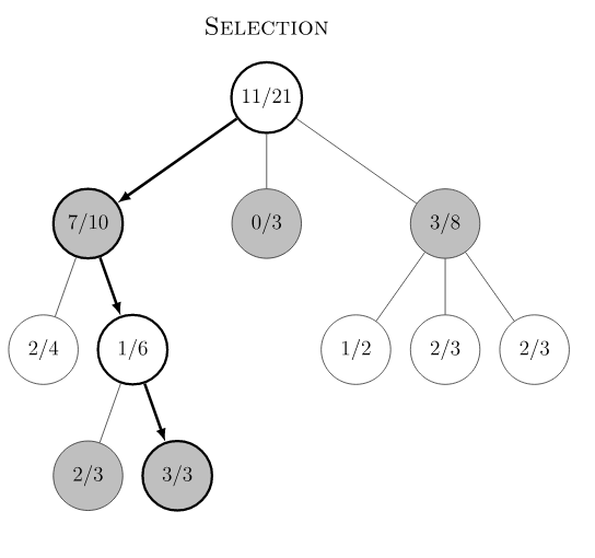
MCTS在playout时遇到已经被展开的节点,会根据selection规则选择子节点,该规则本质上是在所有子节点中选择最大的PUCT值的节点。
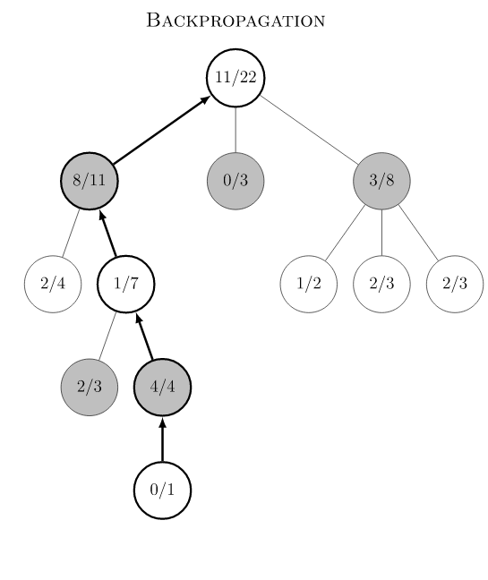
defpropagate_to_root(self, leaf_value: float): """ Updates current node with observed leaf_value and propagates to root node. :param leaf_value: :return: """ if self._parent: self._parent.propagate_to_root(-leaf_value) self._update(leaf_value)
def_update(self, leaf_value: float): """ Updates the node by newly observed leaf_value. :param leaf_value: :return: """ self._visit_num += 1 # new Q is updated towards deviation from existing Q self._Q += 0.5 * (leaf_value - self._Q)
AlphaGo Zero MCTS Player
实现
AlphaGo Zero MCTS
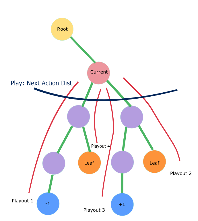
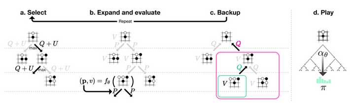
在训练阶段分为如下几个步骤。游戏初始局面下,整个局面树的建立由子节点的不断被探索而丰富起来。AlphaGo
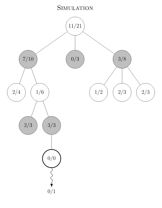
Zero对弈一次即产生了一次完整的游戏开始到结束的动作系列。在对弈过程中的某一游戏局面,需要采样海量的playout,又称MCTS模拟,以此来决定此局面的下一步动作。一次playout可视为在真实游戏状态树的一种特定采样,playout可能会产生游戏结局,生成真实的v值;也可能explore
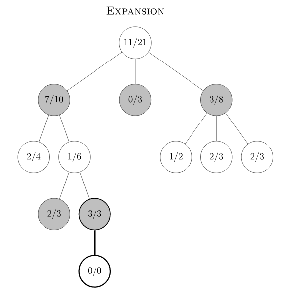
到新的叶子节点,此时v值依赖策略价值网络的输出,目的是利用训练的神经网络来产生高质量的游戏对战局面。每次playout会从当前给定局面递归向下,向下的过程中会遇到下面三种节点情况。
def_next_step_play_act_probs(self, game: ConnectNGame) -> Tuple[List[Pos], ActionProbs]: """ For the given game status, run playouts number of times specified by self._playout_num. Returns the action distribution according to AlphaGo Zero MCTS play formula. :param game: :return: actions and their probability """
for n inrange(self._playout_num): self._playout(copy.deepcopy(game))
defget_action(self, board: PyGameBoard) -> Pos: """ Method defined in BaseAgent. :param board: :return: next move for the given game board. """ return self._get_action(copy.deepcopy(board.connect_n_game))[0]
# the pi defined in AlphaGo Zero paper acts, act_probs = self._next_step_play_act_probs(game) move_probs[list(acts)] = act_probs if self._is_training: # add Dirichlet Noise when training in favour of exploration p_ = (1-epsilon) * act_probs + epsilon * np.random.dirichlet(0.3 * np.ones(len(act_probs))) move = np.random.choice(acts, p=p_) assert move in game.get_avail_pos() else: move = np.random.choice(acts, p=act_probs)
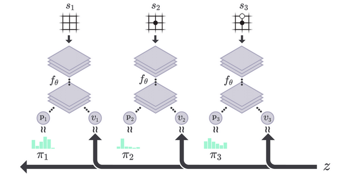
defself_play_one_game(self, game: ConnectNGame) \ -> List[Tuple[NetGameState, ActionProbs, NDArray[(Any), np.float]]]: """ :param game: :return: Sequence of (s, pi, z) of a complete game play. The number of list is the game play length. """
classMCTSAlphaGoZeroPlayer(BaseAgent): def_playout(self, game: ConnectNGame): """ From current game status, run a sequence down to a leaf node, either because game ends or unexplored node. Get the leaf value of the leaf node, either the actual reward of game or action value returned by policy net. And propagate upwards to root node. :param game: """ player_id = game.current_player
# now game state is a leaf node in the tree, either a terminal node or an unexplored node act_and_probs: Iterator[MoveWithProb] act_and_probs, leaf_value = self._policy_value_net.policy_value_fn(game)
ifnot game.game_over: # case where encountering an unexplored leaf node, update leaf_value estimated by policy net to root for act, prob in act_and_probs: game.move(act) child_node = node.expand(act, prob) game.undo() else: # case where game ends, update actual leaf_value to root if game.game_result == ConnectNGame.RESULT_TIE: leaf_value = ConnectNGame.RESULT_TIE else: leaf_value = 1if game.game_result == player_id else -1 leaf_value = float(leaf_value)
# Update leaf_value and propagate up to root node node.propagate_to_root(-leaf_value)
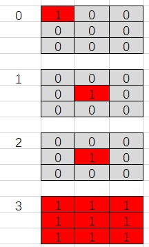
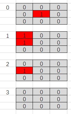
defconvert_game_state(game: ConnectNGame) -> NetGameState: """ Converts game state to type NetGameState as ndarray. :param game: :return: Of shape 4 * board_size * board_size. [0] is current player positions. [1] is opponent positions. [2] is last move location. [3] all 1 meaning move by black player, all 0 meaning move by white. """ state_matrix = np.zeros((4, game.board_size, game.board_size))
if game.action_stack: actions = np.array(game.action_stack) move_curr = actions[::2] move_oppo = actions[1::2] for move in move_curr: state_matrix[0][move] = 1.0 for move in move_oppo: state_matrix[1][move] = 1.0 # indicate the last move location state_matrix[2][actions[-1]] = 1.0 iflen(game.action_stack) % 2 == 0: state_matrix[3][:, :] = 1.0# indicate the colour to play return state_matrix[:, ::-1, :]
AlphaGo Zero 作为Deepmind在围棋领域的最后一代AI
Agent,已经可以达到棋类游戏的终极目标:在只给定游戏规则的情况下,AI
棋手从最初始的随机状态开始,通过不断的自我对弈的强化学习来实现超越以往任何人类棋手和上一代Alpha的能力,并且同样的算法和模型应用到了其他棋类也得出相同的效果。这一篇,从原理上来解析AlphaGo
Zero的运行方式。
AlphaGo Zero
算法由三种元素构成:强化学习(RL)、深度学习(DL)和蒙特卡洛树搜索(MCTS,Monte
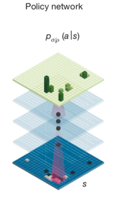
Carlo Tree Search)。核心思想是基于神经网络的Policy
Iteration强化学习,即最终学的是一个深度学习的policy
network,输入是某棋盘局面 s,输出是此局面下可走位的概率分布:\(p(a|s)\)。
在第一代AlphaGo算法中,这个初始policy
network通过收集专业人类棋手的海量棋局训练得来,再采用传统RL 的Monte
Carlo Tree Search Rollout 技术来强化现有的AI对于局面落子(Policy
Network)的判断。Monte Carlo Tree Search Rollout
简单说来就是海量棋局模拟,AI Agent在通过现有的Policy
Network策略完成一次从某局面节点到最终游戏胜负结束的对弈,这个完整的对弈叫做rollout,又称playout。完成一次rollout之后,通过局面树层层回溯到初始局面节点,并在回溯过程中同步修订所有经过的局面节点的统计指标,修正原先policy
network对于落子导致输赢的判断。通过海量并发的棋局模拟来提升基准policy
network,即在各种局面下提高好的落子的\(p(a_{win}|s)\),降低坏的落子的\(p(a_{lose}|s)\)
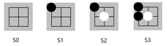
举例如下井字棋局面:
局面s
基准policy network返回 p(s) 如下 \[
p(a|s) =
\begin{align*}
\left\lbrace
\begin{array}{r@{}l}
0.1, & & a = (0,2) \\
0.05, & & a = (1,0) \\
0.5, & & a = (1,1) \\
0.05, & & a = (1,2)\\
0.2, & & a = (2,0) \\
0.05, & & a = (2,1) \\
0.05, & & a = (2,2)
\end{array}
\right.
\end{align*}
\] 通过海量并发模拟后,修订成如下的action概率分布,然后通过policy
iteration迭代新的网络来逼近 \(p'\)
就提高了棋力。 \[
p'(a|s) =
\begin{align*}
\left\lbrace
\begin{array}{r@{}l}
0, & & a = (0,2) \\
0, & & a = (1,0) \\
0.9, & & a = (1,1) \\
0, & & a = (1,2)\\
0, & & a = (2,0) \\
0, & & a = (2,1) \\
0.1, & & a = (2,2)
\end{array}
\right.
\end{align*}
\]
蒙特卡洛树搜索(MCTS)概述
Monte Carlo Tree Search 是Monte Carlo
在棋类游戏中的变种,棋类游戏的一大特点是可以用动作(move)联系的决策树来表示,树的节点数量取决于分支的数量和树的深度。MCTS的目的是在树节点非常多的情况下,通过实验模拟(rollout,
playout)的方式来收集尽可能多的局面输赢情况,并基于这些统计信息,将搜索资源的重点均衡地放在未被探索的节点和值得探索的节点上,减少在大概率输的节点上的模拟资源投入。传统MCTS有四个过程:Selection,
Expansion, Simulation 和Backpropagation。下图是Wikipedia
的例子:
前一代的AlphaGo已经战胜了世界冠军,取得了空前的成就,AlphaGo Zero
的设计目标变得更加General,去除围棋相关的处理和知识,用统一的框架和算法来解决棋类问题。
1. 无人工先验数据
改进之前需要专家棋手对弈数据来冷启动初始棋力
无特定游戏特征工程
无需围棋特定技巧,只包含下棋规则,可以适用到所有棋类游戏
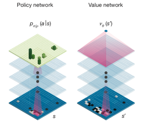
单一神经网络
统一Policy Network和Value
Network,使用一个共享参数的双头神经网络
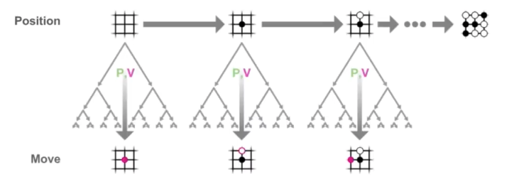
简单树搜索
去除传统MCTS的Rollout
方式,用神经网络来指导MCTS更有效产生搜索策略
搜索空间的两个优化原则
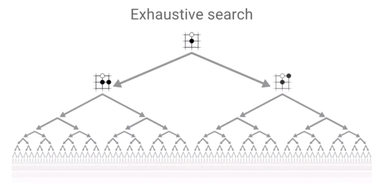
尽管理论上围棋是有解的,即先手必赢、被逼平或必输,通过遍历所有可能局面可以求得解。同理,通过海量模拟所有可能游戏局面,也可以无限逼近所有局面下的真实输赢概率,直至收敛于局面落子的确切最佳结果。但由于围棋棋局的数目远远大于宇宙原子数目,3^361
>>
10^80,因此需要将计算资源有效的去模拟值得探索的局面,例如对于显然的被动局面减小模拟次数,所以如何有效地减小搜索空间是AlphaGo
Zero 需要解决的重大问题。David Silver 在Deepmind
AlphaZero - Mastering Games Without Human Knowledge中提到AlphaGo
Zero 采用两个原则来有效减小搜索空间。
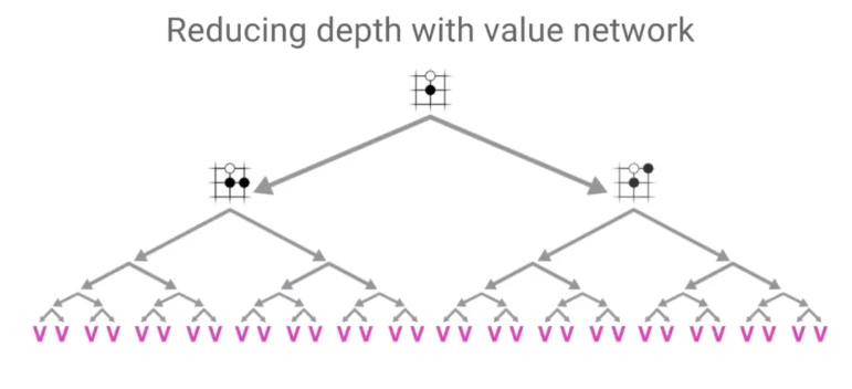
原则1: 通过Value
Network减少搜索的深度
Value Network
通过预测给定局面的value来直接预测最终结果,思想和上一期Minimax DP
策略中直接缓存当前局面的胜负状态一样,减少每次必须靠模拟到最后才能知道当前局面的输赢概率,或者需要多层树搜索才能知道输赢概率。


.png)
.png)