请在桌面浏览器中打开此链接，保证最好的浏览体验

关注公众号后回复 docker-geometric，获取 Docker Image

1
2
3
4
5

# 导入image
docker load < env-torch1.8-geometric.tar

# 运行 jupyter notebook
docker run  -p 8888:8888 -it env-torch1.8-geometric jupyter notebook --allow-root --ip '0.0.0.0' --notebook-dir=/proj

在线代码

• 01 Plot Cora
• 02 Geometric Graph Data Representation
• 03 GCN

公众号系列视频链接

B站视频系列链接

大家一定都用过神奇的 mathpix 服务，它可以方便大家将数学公式图片转换成 Latex 数学公式。现在 MyEncyclopedia 也推出了手机版和桌面版的 mathpix 服务啦！

使用流程 登录服务

1. 关注 MyEncyclopedia 公众号

2. 在公众号对话中回复 ?

3. 点击 AI在线服务

4. 在非微信浏览器中打开链接

5. 登录

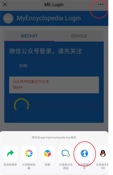
目前提供两种方式。 在国内的小伙伴建议使用微信公众号的方式登录，在国外的朋友们可以使用 Google 账号登录。

5.1 微信登录，按提示在为公众号中输入验证码

5.2 Google登录

使用流程

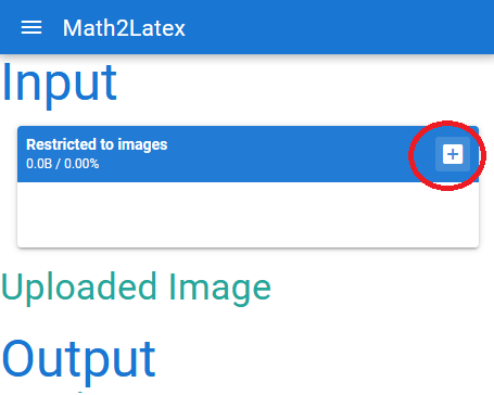
点击右上方 + 选择图片

等待结果

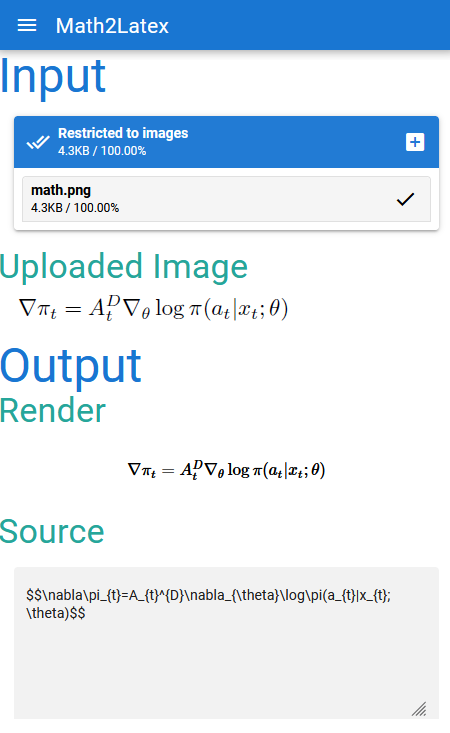
Output Source 为转换的 Latex 源码

Output Render 为转换源码对应的渲染效果

BiliBili

Lecture 1 - Introduction to Unleashing Novel Data at Scale

• Why data accessibility is so central to the advancement of knowledge in economics (with some historical background)
• An overview of the data curation pipeline
  • Step 1: Detect document layouts
  • Step 2: OCR
  • Step 3: Post-processing and database assembly
  • Step 4: Convert information into computable format
• Why is the material covered in this course useful to social scientists?
  • Why there won’t be an app/commercial product capable of end-to-end processing of social science documents anytime soon
  • Why manual data entry often falls short
  • Why our problems differ from those that are the central focus of computer science and the digital humanities
• At its core, deep learning is an optimization problem, which economists are well-trained to understand. It would be really unfortunate if we did not take full advantage of the very powerful methods that deep learning offers, which we are well poised to utilize

Lecture 2 - Why Deep Learning?

This post compares rule-based and deep learning-based approaches to data curation. It discusses their requirements and why rule-based approaches often (but not always) produce disappointing results when applied to social science data.

• An overview of the syllabus (ultimately, the course had a few deviations from the original syllabus, based on student interests; final syllabus posted in the course section of this website)
• There are two distinct approaches to automated data curation
  • Tell the computer how to process the data by defining a set of rules
  • Let the computer learn how to process the data from empirical examples, using deep learning
• Overview of rules, how they are used to process image scans and text, why they often fail, and why they sometimes succeed
• Deep learning, how it contrasts with rule-based approaches, and its requirements
• Does the noise from rule-based approaches really matter?

Lecture 4 - Convolutional Neural Networks

• A brief overview of convolutions
• Benchmark datasets for image classification (following the ConvNent literature requires familiarity with the benchmarks)
• Image classification with a linear classifier (and its shortcomings)
• CNN architectures
  • AlexNet
  • VGG
  • GoogLeNet
  • ResNet
  • ResNext

Lecture 5 - Image Classification; Training Neural Nets

This post covers two topics: using CNNs for image classification (a very useful task) and training neural networks in practice. Much of the information about training neural nets is essential to implementing deep learning-based approaches, whether with CNNs or with some other architecture.

Image Classification

• Loss functions for classification
  • SVM
  • Softmax
• Deep document classification

Training Neural Nets

• Activation functions
• Data pre-processing
• Initialization
• Optimization
• Regularization
• Batch normalization
• Dropout
• Data augmentation
• Transfer learning
• Setting hyperparameters
• Monitoring the learning process

Lecture 6 - Other Computer Vision Problems (Including Object Detection)

This post covers object detection as well as the related problems of semantic segmentation, localization, and instance segmentation. Object detection is core to document image analysis, as it is used to determine the coordinates and classes of different document layout regions. The other problems covered are closely related.

• Semantic segmentation
• Localization
• Object detection
  • Region CNNs
  • Fast R-CNN
  • Faster R-CNN
  • Mask R-CNN
  • Features pyramids
• Instance segmentation
• Other frameworks (YOLO)

Lecture 7 - Object Detection in Practice

• Selecting an object detection model
• Overview of Detectron2
• How-to in D2

Lecture 8 - Labeling and Deep Visualization

Labeling

• Active learning for layout annotation
• Labeling hacks

Deep visualization

• Basic visualization approaches
• Gradient based ascent
• Deep Dream

Lecture 9 - Generative Adversarial Networks

• Overview: supervised and unsupervised learning; generative models
• Generative adversarial networks
• CycleGAN

Lecture 10 - OCR Architecture

• Overview of the OCR problem
• Recurrent neural networks
• LSTMs
• Connectionist temporal classification
• Putting it together

Lecture 11 - OCR and Post-Processing in Practice

This post discusses OCR, both off-the-shelf and how to implement a customized OCR model. It discusses how Layout Parser can be used for end-to-end document image analysis, and provides concrete examples of creating variable domains during post-processing. It also provides an overview of the second half of the knowledge base, which covers NLP.

• Off-the-shelf OCR

• Designing customized OCR

• Putting it altogether (and Layout Parser)

• Creating variable domains

• An overview of the second half of the course (NLP)

Lecture 12 - Models of Words

• Traditional models of words

• Word2Vec

• GloVe

• Evaluation

• Interpreting word vectors

• Problems with word vectors

Lecture 13 - Language Modeling and Other Topics in NLP

This post provides an introduction to language modeling, as well as several other important topics: dependency parsing, named entity recognition (NER), and labeling for NLP. Due to time constraints, the course is able to provide only a very brief introduction to topics like dependency parsing and NER, which have traditionally been quite central questions in NLP research.

• Language Modeling
  • Count based models
  • Bag of words
  • RNN (review)
  • LSTM (review)
• Dependency parsing
• Named entity recognition
• Labeling for NLP

Lecture 14 - Seq2Seq and Machine Translation

Machine translation has pioneered some of the most productive innovations in neural-based NLP and hence is useful to study even for those who care little about machine translation per se. We will focus in particular on seq2seq and attention.

• Statistical machine translation
• Neural machine translation

Lecture 15 - Attention is All You Need

This post introduces the Transformer, a seq2seq model based entirely on attention that has transformed NLP. Given the importance of this paper, there are a bunch of very well-done web resources about it, cited in the lecture and below, that I recommend checking out directly (there are others who have much more of a comparative advantage in presenting seminal NLP papers than I do!).

• A recap of attention

• The Transformer

  • The encoder
    • Encoder self-attention
    • Positional embeddings
    • Add and normalize
  • The decoder
    • Encoder-decoder attention
    • Decoder self-attention
  • Linear and softmax layers
  • Training

Lecture 16 - Transformer-Based Language Models

This post provides an overview of various Transformer-based language models, discussing their architectures and which are best-suited for different contexts.

• Overview
• Contextualized word embeddings
• Models
  • GPT
  • BERT
  • RoBERTa
  • DistilBERT
  • ALBERT
  • T5
  • GPT2/GPT3
  • Transformers XL
  • XLNet
  • Longformer
  • BigBird
• Recap and what to use

Lecture 17 - Understanding Transformers, Visualization, and Sentiment Analysis

This post covers a variety of topics around Transformer-based language models: understanding how Transformer attention works, understanding what information is contained in their embeddings, visualizing embeddings, and using Transformer-based models to conduct sentiment analysis.

• What do Transformer-based models attend to?

• What’s in an embedding?

• Visualizing embeddings

• Sentiment analysis

Lecture 18 - NLP with Noisy Text

• The Canonical Deep NLP Training Corpus
• A definition of noise
• The problem with noise
• Approaches for denoising

Lecture 19 - Retrieval and Question Answering

• Reading comprehension
• Open-domain question answering

Lecture 20 - Zero-Shot and Few-Shot Learning in NLP

• What it means to learn in just a few shots

• Zero-shot and few-shot learning in practice

Lecture 21 - Transformers for Computer Vision

• Transformers for computer vision
• Transformers for image classification
• Transformers for object detection

YouTube

BiliBili

本篇是深度强化学习动手系列文章，自MyEncyclopedia公众号文章深度强化学习之：DQN训练超级玛丽闯关发布后收到不少关注和反馈，这一期，让我们实现目前主流深度强化学习算法PPO来打另一个红白机经典游戏1942。

相关文章链接如下：

强化学习开源环境集

视频论文解读：PPO算法

视频论文解读：组合优化的强化学习方法

解读TRPO论文，深度强化学习结合传统优化方法

解读深度强化学习基石论文：函数近似的策略梯度方法

NES 1942 环境安装

红白机游戏环境可以由OpenAI Retro来模拟，OpenAI Retro还在 Gym 集成了其他的经典游戏环境，包括Atari 2600，GBA，SNES等。

不过，受到版权原因，除了一些基本的rom，大部分游戏需要自行获取rom。

环境准备部分相关代码如下

1

pip install gym-retro

1

python -m retro.import /path/to/your/ROMs/directory/

OpenAI Gym 输入动作类型

在创建 retro 环境时，可以在retro.make中通过参数use_restricted_actions指定 action space，即按键的配置。

1

env = retro.make(game='1942-Nes', use_restricted_actions=retro.Actions.FILTERED)

可选参数如下，FILTERED，DISCRETE和MULTI_DISCRETE 都可以指定过滤的动作，过滤动作需要通过配置文件加载。

1
2
3
4
5
6
7
8

class Actions(Enum):
    """
    Different settings for the action space of the environment
    """
    ALL = 0  #: MultiBinary action space with no filtered actions
    FILTERED = 1  #: MultiBinary action space with invalid or not allowed actions filtered out
    DISCRETE = 2  #: Discrete action space for filtered actions
    MULTI_DISCRETE = 3  #: MultiDiscete action space for filtered actions

DISCRETE和MULTI_DISCRETE 是 Gym 里的 Action概念，它们的基类都是gym.spaces.Space，可以通过 sample()方法采样，下面具体一一介绍。

• Discrete：对应一维离散空间，例如，Discrete(n=4) 表示 [0, 3] 范围的整数。

1
2
3

from gym.spaces import Discrete
space = Discrete(4)
print(space.sample())

输出是

1

3

• Box：对应多维连续空间，每一维的范围可以用 [low，high] 指定。 举例，Box(low=-1.0, high=2, shape=(3, 4,), dtype=np.float32) 表示 shape 是 [3, 4]，每个范围在 [-1, 2] 的float32型 tensor。

1
2
3
4

from gym.spaces import Box
import numpy as np
space = Box(low=-1.0, high=2.0, shape=(3, 4), dtype=np.float32)
print(space.sample())

输出是

1
2
3

[[-0.7538084   0.96901214  0.38641307 -0.05045208]
 [-0.85486996  1.3516271   0.3222616   1.2540635 ]
 [-0.29908678 -0.8970335   1.4869047   0.7007356 ]]

• MultiBinary: 0或1的多维离散空间。例如，MultiBinary([3,2]) 表示 shape 是3x2的0或1的tensor。

  1 2 3

  from gym.spaces import MultiBinary space = MultiBinary([3,2]) print(space.sample())

输出是

1
2
3

[[1 0]
 [1 1]
 [0 0]]

• MultiDiscrete：多维整型离散空间。例如，MultiDiscrete([5,2,2]) 表示三维Discrete空间，第一维范围在 [0-4]，第二，三维范围在[0-1]。

1
2
3

from gym.spaces import MultiDiscrete
space = MultiDiscrete([5,2,2])
print(space.sample())

输出是

1

[2 1 0]

• Tuple：组合成 tuple 复合空间。举例来说，可以将 Box，Discrete，Discrete组成tuple 空间：Tuple(spaces=(Box(low=-1.0, high=1.0, shape=(3,), dtype=np.float32), Discrete(n=3), Discrete(n=2)))

1
2
3
4

from gym.spaces import *
import numpy as np
space = Tuple(spaces=(Box(low=-1.0, high=1.0, shape=(3,), dtype=np.float32), Discrete(n=3), Discrete(n=2)))
print(space.sample())

输出是

1
2

(array([ 0.22640526,  0.75286865, -0.6309239 ], dtype=float32), 0, 1)

• Dict：组合成有名字的复合空间。例如，Dict({'position':Discrete(2), 'velocity':Discrete(3)})

  1 2 3

  from gym.spaces import * space = Dict({'position':Discrete(2), 'velocity':Discrete(3)}) print(space.sample())

输出是

1

OrderedDict([('position', 1), ('velocity', 1)])

NES 1942 动作空间配置

了解了 gym/retro 的动作空间，我们来看看1942的默认动作空间

1
2

env = retro.make(game='1942-Nes')
print("The size of action is: ", env.action_space.shape)

1

The size of action is:  (9,)

表示有9个 Discrete 动作，包括 start, select这些控制键。

从训练1942角度来说，我们希望指定最少的有效动作取得最好的成绩。根据经验，我们知道这个游戏最重要的键是4个方向加上 fire 键。限定游戏动作空间，官方的做法是在创建游戏环境时，指定预先生成的动作输入配置文件。但是这个方式相对麻烦，我们采用了直接指定按键的二进制表示来达到同样的目的，此时，需要设置 use_restricted_actions=retro.Actions.FILTERED。

下面的代码限制了6种按键，并随机play。

1
2
3
4
5
6
7
8
9
10
11
12
13
14
15
16
17
18
19
20
21
22
23
24
25
26
27
28
29
30
31
32
33
34

action_list = [
    # No Operation
    [0, 0, 0, 0, 0, 0, 0, 0, 0, 0, 0, 0],
    # Left
    [0, 0, 0, 0, 0, 0, 1, 0, 0, 0, 0, 0],
    # Right
    [0, 0, 0, 0, 0, 0, 0, 1, 0, 0, 0, 0],
    # Down
    [0, 0, 0, 0, 0, 1, 0, 0, 0, 0, 0, 0],
    # Up
    [0, 0, 0, 0, 1, 0, 0, 0, 0, 0, 0, 0],
    # B
    [1, 0, 0, 0, 0, 0, 0, 0, 0, 0, 0, 0],
]

def random_play(env, action_list, sleep_seconds=0.01):
    env.viewer = None
    state = env.reset()
    score = 0
    for j in range(10000):
        env.render()
        time.sleep(sleep_seconds)
        action = np.random.randint(len(action_list))

        next_state, reward, done, _ = env.step(action_list[action])
        state = next_state
        score += reward
        if done:
            print("Episode Score: ", score)
            env.reset()
            break
            
env = retro.make(game='1942-Nes', use_restricted_actions=retro.Actions.FILTERED)
random_play(env, action_list)

来看看其游戏效果，全随机死的还是比较快。

图像输入处理

一般对于通过屏幕像素作为输入的RL end-to-end训练来说，对图像做预处理很关键。因为原始图像较大，一方面我们希望能尽量压缩图像到比较小的tensor，另一方面又要保证关键信息不丢失，比如子弹的图像不能因为图片缩小而消失。另外的一个通用技巧是将多个连续的frame合并起来组成立体的frame，这样可以有效表示连贯动作。

下面的代码通过 pipeline 将游戏每帧原始图像从shape (224, 240, 3) 转换成 (4, 84, 84)，也就是原始的 width=224，height=240，rgb=3转换成 width=84，height=240，stack_size=4的黑白图像。具体 pipeline为

1. MaxAndSkipEnv：每两帧过滤一帧图像，减少数据量。

2. FrameDownSample：down sample 图像到指定小分辨率 84x84，并从彩色降到黑白。

3. FrameBuffer：合并连续的4帧，形成 (4, 84, 84) 的图像输入

1
2
3
4
5
6
7

def build_env():
    env = retro.make(game='1942-Nes', use_restricted_actions=retro.Actions.FILTERED)
    env = MaxAndSkipEnv(env, skip=2)
    env = FrameDownSample(env, (1, -1, -1, 1))
    env = FrameBuffer(env, 4)
    env.seed(0)
    return env

观察图像维度变换

1
2
3
4
5

env = retro.make(game='1942-Nes', use_restricted_actions=retro.Actions.FILTERED)
print("Initial shape: ", env.observation_space.shape)

env = build_env(env)
print("Processed shape: ", env.observation_space.shape)

确保shape 从 (224, 240, 3) 转换成 (4, 84, 84)

1
2

Initial shape:  (224, 240, 3)
Processed shape:  (4, 84, 84)

FrameDownSample实现如下，我们使用了 cv2 类库来完成黑白化和图像缩放

1
2
3
4
5
6
7
8
9
10
11
12
13
14
15
16
17
18
19
20
21
22
23
24

class FrameDownSample(ObservationWrapper):
    def __init__(self, env, exclude, width=84, height=84):
        super(FrameDownSample, self).__init__(env)
        self.exclude = exclude
        self.observation_space = Box(low=0,
                                     high=255,
                                     shape=(width, height, 1),
                                     dtype=np.uint8)
        self._width = width
        self._height = height

    def observation(self, observation):
        # convert image to gray scale
        screen = cv2.cvtColor(observation, cv2.COLOR_RGB2GRAY)

        # crop screen [up: down, left: right]
        screen = screen[self.exclude[0]:self.exclude[2], self.exclude[3]:self.exclude[1]]

        # to float, and normalized
        screen = np.ascontiguousarray(screen, dtype=np.float32) / 255

        # resize image
        screen = cv2.resize(screen, (self._width, self._height), interpolation=cv2.INTER_AREA)
        return screen

MaxAndSkipEnv，每两帧过滤一帧

1
2
3
4
5
6
7
8
9
10
11
12
13
14
15
16
17
18
19
20
21
22
23

class MaxAndSkipEnv(Wrapper):
    def __init__(self, env=None, skip=4):
        super(MaxAndSkipEnv, self).__init__(env)
        self._obs_buffer = deque(maxlen=2)
        self._skip = skip

    def step(self, action):
        total_reward = 0.0
        done = None
        for _ in range(self._skip):
            obs, reward, done, info = self.env.step(action)
            self._obs_buffer.append(obs)
            total_reward += reward
            if done:
                break
        max_frame = np.max(np.stack(self._obs_buffer), axis=0)
        return max_frame, total_reward, done, info

    def reset(self):
        self._obs_buffer.clear()
        obs = self.env.reset()
        self._obs_buffer.append(obs)
        return obs

FrameBuffer，将最近的4帧合并起来

1
2
3
4
5
6
7
8
9
10
11
12
13
14
15
16

class FrameBuffer(ObservationWrapper):
    def __init__(self, env, num_steps, dtype=np.float32):
        super(FrameBuffer, self).__init__(env)
        obs_space = env.observation_space
        self._dtype = dtype
        self.observation_space = Box(low=0, high=255, shape=(num_steps, obs_space.shape[0], obs_space.shape[1]), dtype=self._dtype)

    def reset(self):
        frame = self.env.reset()
        self.buffer = np.stack(arrays=[frame, frame, frame, frame])
        return self.buffer

    def observation(self, observation):
        self.buffer[:-1] = self.buffer[1:]
        self.buffer[-1] = observation
        return self.buffer

最后，visualize 处理后的图像，同样还是在随机play中，确保关键信息不丢失

1
2
3
4
5
6
7
8
9
10
11
12
13
14
15
16
17
18
19
20
21

def random_play_preprocessed(env, action_list, sleep_seconds=0.01):
    import matplotlib.pyplot as plt

    env.viewer = None
    state = env.reset()
    score = 0
    for j in range(10000):
        time.sleep(sleep_seconds)
        action = np.random.randint(len(action_list))

        plt.imshow(state[-1], cmap="gray")
        plt.title('Pre Processed image')
        plt.pause(sleep_seconds)

        next_state, reward, done, _ = env.step(action_list[action])
        state = next_state
        score += reward
        if done:
            print("Episode Score: ", score)
            env.reset()
            break

matplotlib 动画输出

CNN Actor & Critic

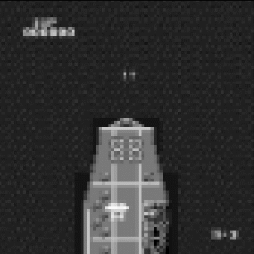
Actor 和 Critic 模型相同，输入是 (4, 84, 84) 的图像，输出是 [0, 5] 的action index。

1
2
3
4
5
6
7
8
9
10
11
12
13
14
15
16
17
18
19
20
21
22
23
24
25
26
27
28

class Actor(nn.Module):
    def __init__(self, input_shape, num_actions):
        super(Actor, self).__init__()
        self.input_shape = input_shape
        self.num_actions = num_actions

        self.features = nn.Sequential(
            nn.Conv2d(input_shape[0], 32, kernel_size=8, stride=4),
            nn.ReLU(),
            nn.Conv2d(32, 64, kernel_size=4, stride=2),
            nn.ReLU(),
            nn.Conv2d(64, 64, kernel_size=3, stride=1),
            nn.ReLU()
        )

        self.fc = nn.Sequential(
            nn.Linear(self.feature_size(), 512),
            nn.ReLU(),
            nn.Linear(512, self.num_actions),
            nn.Softmax(dim=1)
        )

    def forward(self, x):
        x = self.features(x)
        x = x.view(x.size(0), -1)
        x = self.fc(x)
        dist = Categorical(x)
        return dist

PPO核心代码

先计算 \(r_t(\theta)\)，这里采用了一个技巧，对 \(\pi_\theta\) 取 log，相减再取 exp，这样可以增强数值稳定性。

1
2
3
4

dist = self.actor_net(state)
new_log_probs = dist.log_prob(action)
ratio = (new_log_probs - old_log_probs).exp()
surr1 = ratio * advantage

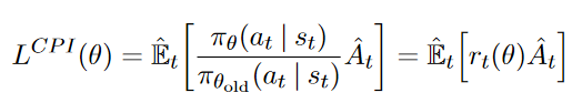
surr1 对应PPO论文中的 \(L^{CPI}\)

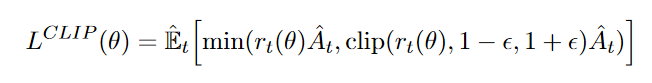
然后计算 surr2，对应 \(L^{CLIP}\) 中的 clip 部分，clip可以由 torch.clamp 函数实现。\(L^{CLIP}\) 则对应 actor_loss。

1
2

surr2 = torch.clamp(ratio, 1.0 - self.clip_param, 1.0 + self.clip_param) * advantage
actor_loss = - torch.min(surr1, surr2).mean()

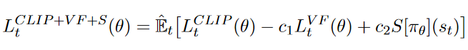
最后，计算总的 loss \(L_t^{CLIP+VF+S}\)，包括 actor_loss，critic_loss 和 policy的 entropy。

1
2
3
4

entropy = dist.entropy().mean()

critic_loss = (return_ - value).pow(2).mean()
loss = actor_loss + 0.5 * critic_loss - 0.001 * entropy

上述完整代码如下

1
2
3
4
5
6
7
8
9
10
11
12
13
14
15
16
17
18
19
20
21
22
23

for _ in range(self.ppo_epoch):
    for state, action, old_log_probs, return_, advantage in sample_batch():
        dist = self.actor_net(state)
        value = self.critic_net(state)

        entropy = dist.entropy().mean()
        new_log_probs = dist.log_prob(action)

        ratio = (new_log_probs - old_log_probs).exp()
        surr1 = ratio * advantage
        surr2 = torch.clamp(ratio, 1.0 - self.clip_param, 1.0 + self.clip_param) * advantage

        actor_loss = - torch.min(surr1, surr2).mean()
        critic_loss = (return_ - value).pow(2).mean()

        loss = actor_loss + 0.5 * critic_loss - 0.001 * entropy

        # Minimize the loss
        self.actor_optimizer.zero_grad()
        self.critic_optimizer.zero_grad()
        loss.backward()
        self.actor_optimizer.step()
        self.critic_optimizer.step()

补充一下 GAE 的计算，advantage 根据公式

可以转换成如下代码

1
2
3
4
5
6
7
8
9

def compute_gae(self, next_value):
    gae = 0
    returns = []
    values = self.values + [next_value]
    for step in reversed(range(len(self.rewards))):
        delta = self.rewards[step] + self.gamma * values[step + 1] * self.masks[step] - values[step]
        gae = delta + self.gamma * self.tau * self.masks[step] * gae
        returns.insert(0, gae + values[step])
    return returns

外层 Training 代码

外层调用代码基于随机 play 的逻辑，agent.act()封装了采样和 forward prop，agent.step() 则封装了 backprop 和参数学习迭代的逻辑。

1
2
3
4
5
6
7
8
9
10
11
12
13
14
15
16

for i_episode in range(start_epoch + 1, n_episodes + 1):
    state = env.reset()
    score = 0
    timestamp = 0

    while timestamp < 10000:
        action, log_prob, value = agent.act(state)
        next_state, reward, done, info = env.step(action_list[action])
        score += reward
        timestamp += 1

        agent.step(state, action, value, log_prob, reward, done, next_state)
        if done:
            break
        else:
            state = next_state

训练结果

让我们来看看学习的效果吧，注意我们的飞机学到了一些关键的技巧，躲避子弹；飞到角落尽快击毙敌机；一定程度预测敌机出现的位置并预先走到位置。

YouTube

BiliBili

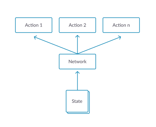
Policy gradient 定理作为现代深度强化学习的基石，同时也是actor-critic的基础，重要性不言而喻。但是它的推导和理解不是那么浅显，不同的资料中又有着众多形式，不禁令人困惑。本篇文章MyEncyclopedia试图总结众多资料背后的一些相通的地方，并写下自己的一些学习理解心得。

引入 Policy Gradient

那么问题来了，首先一个如何定义 \(J(\theta)\)，其次，如何求出或者估计 $ J()$。

第一个问题比较直白，用value function或者广义的expected return都可以。

这里列举一些常见的定义。对于episodic 并且初始都是 \(s_0\)状态的情况，直接定义成v值，即Sutton教程中的episodic情况下的定义

其中，状态平稳分布 \(d^{\pi}(s)\) 定义为

即$ $ 是一次trajectory，服从以 \(\theta\) 作为参数的随机变量

\(J(\theta)\) 对于所有的可能的 \(\tau\) 求 expected return。这种视角下对于finite 和 infinite horizon来说也有变形。

当环境dynamics未知时，如何再去求 $ J()$ 呢。还有就是如果涉及到状态的分布也是取决于环境dynamics的，计算 $ J()$ 也面临同样的问题。

幸好，policy gradient定理完美的解答了上述问题。我们先来看看它的表述内容。

Policy Gradient Theorem

Policy Gradient 定理的伟大之处在于等式右边并没有 \(d^{\pi}(s)\)，或者环境transition model \(p\left(s^{\prime}, r \mid s, a\right)\)！同时，等式右边变换成了最利于统计采样的期望形式，因为期望可以通过样本的平均来估算。

但是，这里必须注意的是action space的期望并不是基于 $(a S_{t}, ) $ 的权重的，因此，继续改变形式，引入 action space的 on policy 权重 $(a S_{t}, ) $ ，得到 2.3式。

将 \(q_{\pi}\)替换成 \(G_t\)，由于

得到2.5式

Policy Gradient Theorem - Trajectory Form

和监督学习的联系

Policy Gradient中的 \(\nabla_{\theta} \log \pi\) 广泛存在在机器学习范畴中，被称为 score function gradient estimator。RL 在supervised learning settings 中有 imitation learning，即通过专家的较优stochastic policy \(\pi_{\theta}(a|s)\) 收集数据集

对照Policy Graident RL，on-policy \(\pi_{\theta}(a|s)\) 产生数据集

目标是最大化on-policy \(\pi_{\theta}\) 分布下的expected return

对比 4.3 和 4.2，发现此时4.3中只多了一个权重系数 \(G_n\)。

关于 $G_{n} {} {}(a_{n} s_{n}) $ 或者 \(G_{t} \frac{\nabla \pi\left(A_{t} \mid S_{t}, \boldsymbol{\theta}_{t}\right)}{\pi\left(A_{t} \mid S_{t}, \boldsymbol{\theta}_{t}\right)}\) 有一些深入的理解。

Policy Gradient 工作的机制大致如下

首先，根据现有的 on-policy \(\pi_{\theta}\) 采样出一些动作 action 产生trajectories，这些trajectories最终得到反馈 \(R(\tau)\)

最后，由于采样到的action分布服从于\(a \sim \pi_{\theta}(a)\) ，除掉 \(\pi_{\theta}\) ：

\(G_{t} \frac{\nabla \pi\left(A_{t} \mid S_{t}, \boldsymbol{\theta}_{t}\right)}{\pi\left(A_{t} \mid S_{t}, \boldsymbol{\theta}_{t}\right)}\)

此时，采样的均值可以去无偏估计2.2式中的Expectation。

上一期 MyEncyclopedia公众号文章 从Q-Learning 演化到 DQN，我们从原理上讲解了DQN算法，这一期，让我们通过代码来实现任天堂游戏机中经典的超级玛丽的自动通关吧。本文所有代码在 https://github.com/MyEncyclopedia/reinforcement-learning-2nd/tree/master/super_mario。

DQN 算法回顾

上期详细讲解了DQN中的两个重要的技术：Target Network 和 Experience Replay，正是有了它们才使得 Deep Q Network在实战中容易收敛，以下是Deepmind 发表在Nature 的 Human-level control through deep reinforcement learning 的完整算法流程。

超级玛丽 NES OpenAI 环境

安装基于OpenAI gym的超级玛丽环境执行下面的 pip 命令即可。

1

pip install gym-super-mario-bros

我们先来看一下游戏环境的输入和输出。下面代码采用随机的action来和游戏交互。有了 组合游戏系列3: 井字棋、五子棋的OpenAI Gym GUI环境 对于OpenAI Gym 接口的介绍，现在对于其基本的交互步骤已经不陌生了。

1
2
3
4
5
6
7
8
9
10
11
12
13
14
15
16
17
18
19
20
21
22

import gym_super_mario_bros
from random import random, randrange
from gym_super_mario_bros.actions import RIGHT_ONLY
from nes_py.wrappers import JoypadSpace
from gym import wrappers

env = gym_super_mario_bros.make('SuperMarioBros-v0')
env = JoypadSpace(env, RIGHT_ONLY)

# Play randomly
done = False
env.reset()

step = 0
while not done:
    action = randrange(len(RIGHT_ONLY))
    state, reward, done, info = env.step(action)
    print(done, step, info)
    env.render()
    step += 1

env.close()

游戏render效果如下

。。。

注意我们在游戏环境初始化的时候用了参数 RIGHT_ONLY，它定义成五种动作的list，表示仅使用右键的一些组合，适用于快速训练来完成Mario第一关。

1
2
3
4
5
6
7

RIGHT_ONLY = [
    ['NOOP'],
    ['right'],
    ['right', 'A'],
    ['right', 'B'],
    ['right', 'A', 'B'],
]

观察一些 info 输出内容，coins表示金币获得数量，flag_get 表示是否取得最后的旗子，time 剩余时间，以及 Mario 大小状态和所在的 x，y位置。

1
2
3
4
5
6
7
8
9
10
11
12

{
   "coins":0,
   "flag_get":False,
   "life":2,
   "score":0,
   "stage":1,
   "status":"small",
   "time":381,
   "world":1,
   "x_pos":594,
   "y_pos":89
}

游戏图像处理

Deep Reinforcement Learning 一般是 end-to-end learning，意味着游戏的 screen image 作为observation直接视为真实状态，喂给神经网络训练。于此相反的另一种做法是，通过游戏环境拿到内部状态，例如所有相关物品的位置和属性作为模型输入。这两种方式的区别有两点。第一点，用观察到的屏幕像素代替真正的状态 s，在partially observable 的环境时可能因为 non-stationarity 导致无法很好的工作，而拿内部状态利用了额外的作弊信息，在partially observable环境中也可以工作。第二点，第一种方式屏幕像素维度比较高，输入数据量大，需要神经网络的大量训练拟合，第二种方式，内部真实状态往往维度低得多，训练起来很快，但缺点是因为除了内部状态往往还需要游戏相关规则作为输入，因此generalization能力不如前者强。

这里，我们当然采样屏幕像素的 end-to-end 方式了，自然首要任务是将游戏帧图像有效处理。超级玛丽游戏环境的屏幕输出是 (240, 256, 3) shape的 numpy array，通过下面一系列的转换，尽可能的在不影响训练效果的情况下减小采样到的数据量。

1. MaxAndSkipFrameWrapper：每4个frame连在一起，采取同样的动作，降低frame数量。

2. FrameDownsampleWrapper：将原始的 (240, 256, 3) down sample 到 (84, 84, 1)

3. ImageToPyTorchWrapper：转换成适合 pytorch 的 (1, 84, 84) shape

4. FrameBufferWrapper：保存最后4次屏幕采样

5. NormalizeFloats：Normalize 成 [0., 1.0] 的浮点值

1
2
3
4
5
6
7
8
9

def wrap_environment(env_name: str, action_space: list) -> Wrapper:
    env = make(env_name)
    env = JoypadSpace(env, action_space)
    env = MaxAndSkipFrameWrapper(env)
    env = FrameDownsampleWrapper(env)
    env = ImageToPyTorchWrapper(env)
    env = FrameBufferWrapper(env, 4)
    env = NormalizeFloats(env)
    return env

CNN 模型

模型比较简单，三个卷积层后做 softmax输出，输出维度数为离散动作数。act() 采用了epsilon-greedy 模式，即在epsilon小概率时采取随机动作来 explore，大于epsilon时采取估计的最可能动作来 exploit。

1
2
3
4
5
6
7
8
9
10
11
12
13
14
15
16
17
18
19
20
21
22
23
24
25
26
27
28
29
30
31
32
33

class DQNModel(nn.Module):
    def __init__(self, input_shape, num_actions):
        super(DQNModel, self).__init__()
        self._input_shape = input_shape
        self._num_actions = num_actions

        self.features = nn.Sequential(
            nn.Conv2d(input_shape[0], 32, kernel_size=8, stride=4),
            nn.ReLU(),
            nn.Conv2d(32, 64, kernel_size=4, stride=2),
            nn.ReLU(),
            nn.Conv2d(64, 64, kernel_size=3, stride=1),
            nn.ReLU()
        )

        self.fc = nn.Sequential(
            nn.Linear(self.feature_size, 512),
            nn.ReLU(),
            nn.Linear(512, num_actions)
        )

    def forward(self, x):
        x = self.features(x).view(x.size()[0], -1)
        return self.fc(x)

    def act(self, state, epsilon, device):
        if random() > epsilon:
            state = torch.FloatTensor(np.float32(state)).unsqueeze(0).to(device)
            q_value = self.forward(state)
            action = q_value.max(1)[1].item()
        else:
            action = randrange(self._num_actions)
        return action

Experience Replay 缓存

实现采用了 Pytorch CartPole DQN 的官方代码，本质是一个最大为 capacity 的 list 保存采样的 (s, a, r, s', is_done) 五元组。

1
2
3
4
5
6
7
8
9
10
11
12
13
14
15
16
17
18
19
20

Transition = namedtuple('Transition', ('state', 'action', 'reward', 'next_state', 'done'))

class ReplayMemory:

    def __init__(self, capacity):
        self.capacity = capacity
        self.memory = []
        self.position = 0

    def push(self, *args):
        if len(self.memory) < self.capacity:
            self.memory.append(None)
        self.memory[self.position] = Transition(*args)
        self.position = (self.position + 1) % self.capacity

    def sample(self, batch_size):
        return random.sample(self.memory, batch_size)

    def __len__(self):
        return len(self.memory)

DQNAgent

我们将 DQN 的逻辑封装在 DQNAgent 类中。DQNAgent 成员变量包括两个 DQNModel，一个ReplayMemory。

train() 方法中会每隔一定时间将 Target Network 的参数同步成现行Network的参数。在td_loss_backprop()方法中采样 ReplayMemory 中的五元组，通过minimize TD error方式来改进现行 Network 参数 \(\theta\)。Loss函数为：

\[ L\left(\theta_{i}\right)=\mathbb{E}_{\left(s, a, r, s^{\prime}\right) \sim \mathrm{U}(D)}\left[\left(r+\gamma \max _{a^{\prime}} Q_{target}\left(s^{\prime}, a^{\prime} ; \theta_{i}^{-}\right)-Q\left(s, a ; \theta_{i}\right)\right)^{2}\right] \]

1
2
3
4
5
6
7
8
9
10
11
12
13
14
15
16
17
18
19
20
21
22
23
24
25
26
27
28
29
30
31
32
33
34
35
36
37
38
39

class DQNAgent():

    def act(self, state, episode_idx):
        self.update_epsilon(episode_idx)
        action = self.model.act(state, self.epsilon, self.device)
        return action

    def process(self, episode_idx, state, action, reward, next_state, done):
        self.replay_mem.push(state, action, reward, next_state, done)
        self.train(episode_idx)

    def train(self, episode_idx):
        if len(self.replay_mem) > self.initial_learning:
            if episode_idx % self.target_update_frequency == 0:
                self.target_model.load_state_dict(self.model.state_dict())
            self.optimizer.zero_grad()
            self.td_loss_backprop()
            self.optimizer.step()

    def td_loss_backprop(self):
        transitions = self.replay_mem.sample(self.batch_size)
        batch = Transition(*zip(*transitions))

        state = Variable(FloatTensor(np.float32(batch.state))).to(self.device)
        action = Variable(LongTensor(batch.action)).to(self.device)
        reward = Variable(FloatTensor(batch.reward)).to(self.device)
        next_state = Variable(FloatTensor(np.float32(batch.next_state))).to(self.device)
        done = Variable(FloatTensor(batch.done)).to(self.device)

        q_values = self.model(state)
        next_q_values = self.target_net(next_state)

        q_value = q_values.gather(1, action.unsqueeze(-1)).squeeze(-1)
        next_q_value = next_q_values.max(1)[0]
        expected_q_value = reward + self.gamma * next_q_value * (1 - done)

        loss = (q_value - expected_q_value.detach()).pow(2)
        loss = loss.mean()
        loss.backward()

外层 Training 代码

最后是外层调用代码，基本和以前文章一样。

1
2
3
4
5
6
7
8
9
10
11
12
13
14
15
16

def train(env, args, agent):
    for episode_idx in range(args.num_episodes):
        episode_reward = 0.0
        state = env.reset()

        while True:
            action = agent.act(state, episode_idx)
            if args.render:
                env.render()
            next_state, reward, done, stats = env.step(action)
            agent.process(episode_idx, state, action, reward, next_state, done)
            state = next_state
            episode_reward += reward
            if done:
                print(f'{episode_idx}: {episode_reward}')
                break

本篇是TSP问题从DP算法到深度学习系列第四篇，这一篇我们会详细举例并比较在 seq-to-seq 或者Markov Chain中的一些常见的搜索概率最大的状态序列的算法。这些方法在深度学习的seq-to-seq 中被用作decoding。在第五篇中，我们使用强化学习时也会使用了本篇中讲到的方法。

• 第一篇: 递归DP方法 AC AIZU TSP问题

• 第二篇: 二维空间TSP数据集及其DP解法

• 第三篇: 深度学习 Pointer Networks 的 Pytorch实现

• 第四篇: 搜寻最有可能路径：Viterbi算法和其他

• 第五篇: 深度强化学习无监督算法的 Pytorch实现

马尔科夫链问题

在 seq-to-seq 问题中，我们经常会遇到需要从现有模型中找概率最大的可能状态序列。这类问题在机器学习算法和控制领域广泛存在，抽象出来可以表达成马尔可夫链模型：给定初始状态的分布和系统的状态转移方程（称为系统动力，dynamics），找寻最有可能的状态序列。

举个例子，假设系统有 \(n\) 个状态，初始状态由 $s_0 = [0.35, 0.25, 0.4] $ 指定，表示初始时三种状态的分布为 0.35，0.25和0.4。

状态转移矩阵由 \(T\) 表达，其中 $ T[i][j]$ 表示从状态 \(i\) 到状态 \(j\) 的概率。注意下面的矩阵 \(T\) 每行的和为 1.0，对应了从任意状态出发，下一时刻的所有可能转移概率和为1。 \[ T= \begin{matrix} & \begin{matrix}0&1&2\end{matrix} \\\\ \begin{matrix}0\\\\1\\\\2\end{matrix} & \begin{bmatrix}0.3&0.6&0.1\\\\0.4&0.2&0.4\\\\0.3&0.3&0.4\end{bmatrix}\\\\ \end{matrix} \]

至此，系统的所有参数都定下来了。接下去的各个时刻的状态分布可以通过矩阵乘法来算得。比如，记\(s_1\) 为 \(t_1\) 时刻状态分布，计算方法为 \(s_0\) 乘以 \(T\)，动画如下：

\(s_1\) 数值计算结果如下。

\[ s_1 = \begin{bmatrix}0.35& 0.25& 0.4\end{bmatrix} \begin{matrix} \begin{bmatrix}0.3&0.6&0.1\\\\0.4&0.2&0.4\\\\0.3&0.3&0.4\end{bmatrix}\\\\ \end{matrix} = \begin{bmatrix}0.325& 0.35& 0.255\end{bmatrix} \] 矩阵左乘行向量可以理解为矩阵每一行的线性组合，直觉上理解为下一时刻的状态分布是上一时刻初始状态分布乘以转移关系的线性组合。 \[ \begin{bmatrix}0.35& 0.25& 0.4\end{bmatrix} \begin{matrix} \begin{bmatrix}0.3&0.6&0.1\\\\0.4&0.2&0.4\\\\0.3&0.3&0.4\end{bmatrix}\\\\ \end{matrix} = 0.35 \times \begin{bmatrix}0.35& 0.6& 0.1\end{bmatrix} + 0.25 \times \begin{bmatrix}0.4& 0.2& 0.4\end{bmatrix} + 0.4 \times \begin{bmatrix}0.3& 0.3& 0.4\end{bmatrix} \] 同样的，后面每一个时刻都可以由上一个状态分布向量乘以 \(T\)，当然这里我们假设每个时刻的转移矩阵是不变的。当然，问题也可以是每个时刻都有不同的转移矩阵来定义，例如深度学习 seq-to-seq 模型。当然，这个设定的变化不会影响搜索最可能状态序列的算法。出于简单考虑，本篇中我们假定所有时刻的状态转移矩阵都是 \(T\)。

下面我们通过多种算法来找出由上述参数定义的系统中前三个时刻的最有可能序列，即概率最大的 \(s_0 \rightarrow s_1 \rightarrow s_2\)。

令 \(L\) 是阶段数，\(N\) 是每个阶段的状态数，则我们的例子中 \(L=N=3\) 。并且，总共有 \(N^L\) 种不同的路径。

穷竭搜索

若给定一条路径，计算特定路径的概率是很直接的，例如，若给定路径为 \(2(s_0) \rightarrow 1(s_1) \rightarrow 2(s_2)\)，则这条路径的概率为

\[ p(2 \rightarrow 1 \rightarrow 2) = s_0[2] \times T[2][1] \times T[1][2] = 0.4 \times 0.3 \times 0.4 = 0.048 \]

因此，我们可以通过枚举所有 \(N^L\) 条路径并计算每条路径的概率来找到最有可能的状态序列。

下面是Python 3的穷竭搜索代码，输出为最有可能的概率及其路径。样例问题的输出为 0.084 和状态序列 \(0 \rightarrow 1 \rightarrow 2\)。

1
2
3
4
5
6
7
8
9
10
11
12
13
14
15
16
17
18
19

def search_brute_force(initial: List, transition: List, L: int) -> Tuple[float, Tuple]:
    from itertools import combinations_with_replacement
    v = [0, 1, 2]
    path_all = combinations_with_replacement(v, L)

    max_prop = 0.0
    max_route = None
    prob = 0.0
    for path in list(path_all):
        for idx, v in enumerate(path):
            if idx == 0:
                prob = initial[v]  # reset to initial state
            else:
                prev_v = path[idx-1]
                prob *= transition[prev_v][v]
        if prob > max_prop:
            max_prop = max(max_prop, prob)
            max_route = path
    return max_prop, max_route

贪心搜索

穷竭搜索一定会找到最有可能的状态序列，但是算法复杂度是指数级的 \(O(N^L)\)。一种最简化的策略是，每一时刻都只选取下一时刻最可能的状态，显然这种策略没有考虑全局最优，只考虑下一步最优，因此称为贪心策略。当然，贪心策略虽然牺牲全局最优解但是换取了很快的时间复杂度。贪心搜索算法动画如下。

Python 3 实现中我们利用了 numpy 类库，主要是 np.argmax() 可以让代码简洁。代码本质上是两重循环，（一层循环是np.argmax中），对应时间算法复杂度是 \(O(N\times L)\)。

1
2
3
4
5
6
7
8
9
10
11
12
13
14
15
16
17
18

def search_greedy(initial: List, transition: List, L: int) -> Tuple[float, Tuple]:
    import numpy as np
    max_route = []
    max_prop = 0.0
    states = np.array(initial)

    prev_max_v = None
    for l in range(0, L):
        max_v = np.argmax(states)
        max_route.append(max_v)
        if l == 0:
            max_prop = initial[max_v]
        else:
            max_prop = max_prop * transition[prev_max_v][max_v]
        states = max_prop * states
        prev_max_v = max_v

    return max_prop, max_route

Beam 搜索

贪心策略只考虑了下一步的最大概率状态，若我们改进一下贪心策略，将下一步的最大 \(k\) 个状态保留下来就是beam 搜索了。具体来说， \(k\) beam search表示每个阶段保留 \(k\) 个最大概率路径，下一阶段扩展这 \(k\) 条路径至 \(k \times N\) 条路径再选取最大的top k。以上例来说，选取\(k=2\)，则初始 \(s_0\)时选取最大概率的两种状态 0和 2，下一阶段 \(s_1\)，计算以0和2开始的共 \(2 \times 3\) 条路径，并保留其中最大概率的两条，如此往复。显然，beam search也无法找到全局最优解，但是它能以线性时间复杂度探索更多的路径空间。

以下是Python 3 的代码实现，利用了 PriorityQueue 选取 \(k\) 路径。由于PriorityQueue 无法自定义比较关系，我们定义了 @total_ordering 标注的类来实现比较关心。时间算法复杂度是 \(O(k\times N \times L)\) 。

1
2
3
4
5
6
7
8
9
10
11
12
13
14
15
16
17
18
19
20
21
22
23
24
25
26
27
28
29
30
31
32
33
34
35
36
37
38

def search_beam(initial: List, transition: List, L: int, K: int) -> Tuple[float, Tuple]:
    N = len(initial)
    from queue import PriorityQueue
    current_q = PriorityQueue()
    next_q = PriorityQueue()

    from functools import total_ordering
    @total_ordering
    class PQItem(object):
        def __init__(self, prob, route):
            self.prob = prob
            self.route = route
            self.last_v = int(route[-1])

        def __eq__(self, other):
            return self.prob == other.prob

        def __lt__(self, other):
            return self.prob > other.prob

    for v in range(N):
        next_q.put(PQItem(initial[v], str(v)))

    for l in range(1, L):
        current_q = next_q
        next_q = PriorityQueue()
        k = K
        while not current_q.empty() and k > 0:
            item = current_q.get()
            prob, route, prev_v = item.prob, item.route, item.last_v
            k -= 1
            for v in range(N):
                nextItem = PQItem(prob * transition[prev_v][v], route + str(v))
                next_q.put(nextItem)

    max_item = next_q.get()

    return max_item.prob, list(map(lambda x: int(x), max_item.route))

Viterbi 动态规划

和之前TSP 动态规划算法的思想一样，最有可能状态路径问题解法有可以将指数时间复杂度 \(O(N^L)\) 降到多项式时间复杂度 \(O(L \times N \times N)\) 的算法，就是大名鼎鼎的 Viterbi 算法（维特比算法）。核心思想是在每个阶段，用数组保存每个状态结尾路径的阶段最大概率（及其对应路径）。在不考虑优化空间的情况下，我们开一个二维数组 \(dp[][]\)，第一维表示阶段序号，第二维表示状态序号。例如，\(dp[1][0]\) 是 \(s_1\) 阶段时以状态0结尾的所有路径中的最大概率，即 \[ dp[1][0] = \max \\{s_0[0] \rightarrow s_1[0], s_0[1] \rightarrow s_1[0], s_0[2] \rightarrow s_1[0]\\} \]

实现代码中没有返回路径本身而只是其概率值，目的是通过简洁的三层循环来表达算法精髓。

1
2
3
4
5
6
7
8
9
10
11

def search_dp(initial: List, transition: List, L: int) -> float:
    N = len(initial)
    dp = [[0.0 for c in range(N)] for r in range(L)]
    dp[0] = initial[:]

    for l in range(1, L):
        for v in range(N):
            for prev_v in range(N):
                dp[l][v] = max(dp[l][v], dp[l - 1][prev_v] * transition[prev_v][v])

    return max(dp[L-1])

概率采用

以上所有的算法都是确定性的。在NLP 深度学习decoding 时候会带来一个问题：确定性容易导致生成重复的短语或者句子。比如，确定性算法很容易生成如下句子。

1

This is the best of best of best of ...

1
2
3
4
5
6
7
8
9
10
11
12
13
14
15
16

def search_prob_greedy(initial: List, transition: List, L: int) -> Tuple[float, Tuple]:
    import random
    N = len(initial)
    max_route = []
    max_prop = 0.0
    vertices = [i for i in range(N)]
    prob = initial[:]

    for l in range(0, L):
        v_lst = random.choices(vertices, prob)
        v = v_lst[0]
        max_route.append(v)
        max_prop = prob[v]
        prob = [prob[v] * transition[v][v_target] for v_target in range(N)]

    return max_prop, max_route

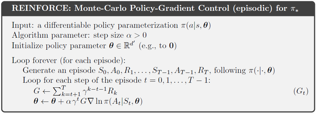
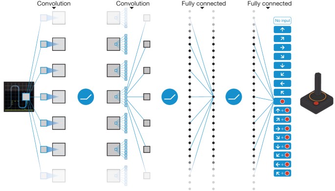
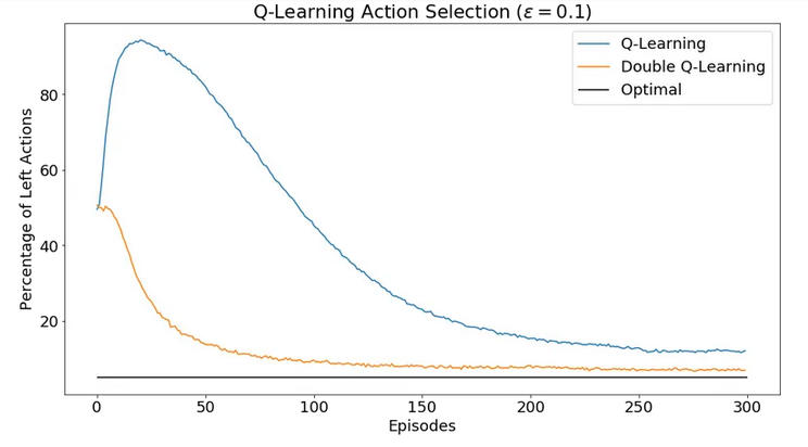
上一期 MyEncyclopedia公众号文章 SARSA、Q-Learning和Expected SARSA时序差分算法训练CartPole中，我们通过CartPole的OpenAI Gym环境实现了Q-learning算法，这一期，我们将会分析Q-learning算法面临的maximization bias 问题和提出double learning算法来改进。接着，我们将tabular Q-learning算法扩展到用带参函数来近似 Q(s, a)，这就是Deepmind 在2015年Nature上发表的Deep Q Network （DQN）思想：用神经网络结合Q-learning算法实现超越人类玩家打Atari游戏的水平。

Q-Learning 回顾

在SARSA、Q-Learning和Expected SARSA时序差分算法训练CartPole 中，我们实现了同样基于 \(\epsilon\)-greedy 策略的Q-learning算法和SARSA算法，两者代码上的区别确实不大，但本质上Q-learning是属于 off-policy 范畴而 SARSA却属于 on-policy 范畴。一种理解方式是，Q-learning相比于SARSA少了第二次从 \(\epsilon\)-greedy 策略采样出下一个action，即S, A, R', S', A' 五元组中最后一个A'，而直接通过max操作去逼近 \(q^{*}\)。如此，Q-learning并没有像SARSA完成一次完整的GPI（Generalized Policy Iteration），缺乏on-policy的策略迭代的特点，故而 Q-learning 属于off-policy方法。我们也可以从另一个角度来分析两者的区别。注意到这两个算法不是一定非要使用 \(\epsilon\)-greedy 策略的。对于Q-learning来说，完全可以使用随机策略，理论上已经证明，只要保证每个action以后依然有几率会被探索下去，Q-learning 最终会收敛到最优策略。Q-learning使用 \(\epsilon\)-greedy 是为了能快速收敛。对于SARSA算法来说，则无法使用随机策略，因为随机策略无法形成策略提升。而 \(\epsilon\)-greedy 策略却可以形成策略迭代，完成策略提升，当然，\(\epsilon\)-greedy 策略在 SARSA 算法中也可以保证快速收敛。因此，尽管两者都使用 \(\epsilon\)-greedy 策略再借由环境产生reward和state，它们的作用并非完全一样。至此，我们可以体会到on-policy和off-policy本质的区别。

收敛条件

一种方式是将 \(\alpha\)设置成 (s, a)访问次数的倒数：\(\alpha_{n}(s,a) = 1/ n(s,a )\)

则整体更新公式为

\[ Q(s,a) \leftarrow Q(s,a) + \alpha_n(s, a)[R+\gamma \max_{a^{\prime}}Q(s^{\prime}, a^{\prime}) - Q(s, a)] \]

Q-Learning 最大化偏差问题

Q-Learning 会产生最大化偏差问题（Maximization Bias，在Sutton 教材6.7节），它的原因是用估计值中取最大值去估计真实值中最大是有偏的。这个可以做如下试验来模拟，若有5个 [-3, 3] 的离散均匀分布 \(d_i\)，\(\max(\mathbb{E}[d_i]) = 0\)，但是若我们用单批采样 \(x_i \sim d_i\)来估算 \(\mathbb{E}[d_i]\)在取max的话，\(\mathbb{E}[{\max(x_i)]}\) 是有bias的。但是如果我们将这个过程分解成选择最大action和评估其值两步，每一步用独立的采样集合就可以做到无偏，这个改进方法称为double learning。具体过程为第一步在\(Q_1\)集合中找到最大的action，第二步在\(Q_2\)中返回此action值，即：

则无限模拟后结果是无偏的：\(\mathbb{E}[Q_2(A^{\star})] = q(A^{\star})\) 下面是简单模拟试验两种方法的均值比较

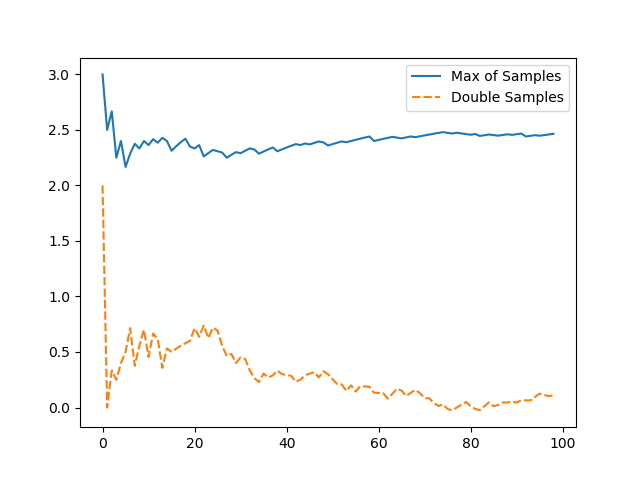
试验完整代码如下

1
2
3
4
5
6
7
8
9
10
11
12
13
14
15
16
17
18
19
20
21
22
23
24
25
26
27
28
29
30
31
32

import random
from math import floor
import numpy as np
import pandas as pd
import seaborn as sns


def uniform(a: int, b: int) -> int:
    u = random.random()
    return a + floor((b - a + 1) * u)


if __name__ == "__main__":
    total_max_bias = 0
    avgs_max_bias = []
    total_double_sampling = 0
    avgs_double_sampling = []

    for e in range(1, 100):
        samples = np.array([uniform(-3, 3) for _ in range(5)])
        max_sample = max(samples)
        total_max_bias += max_sample
        avgs_max_bias.append(total_max_bias / e)

        samples2 = np.array([uniform(-3, 3) for _ in range(5)])
        total_double_sampling += samples2[np.argmax(samples)]
        avgs_double_sampling.append(total_double_sampling / e)

    df = pd.DataFrame({'Max of Samples': avgs_max_bias, 'Double Samples': avgs_double_sampling})
    import matplotlib.pyplot as plt
    sns.lineplot(data=df)
    plt.show()

回到Q-learning 中使用的 \(\epsilon\)-greedy策略，Q-learning可以保证随着\(\epsilon\) 的减小，最大化偏差会 asymptotically 趋近于真实值，但是double learning 可以更快地趋近于真实值。

下面是Sutton 强化学习第二版6.7节中完整的Double Q-learning算法。

更详细内容，可以参考 Hado V. Hasselt 的 Double Q-learning paper [3]。

Gradient Q-Learning

Tabular Q-learning由于受制于维度爆炸，无法扩展到高维状态空间，一般近似解决方案是用 approximating function来逼近Q函数。即我们将状态抽象出一组特征 \(s = \vec x= [x_1, x_2, ..., x_n]^T\)，Q 用一个 x 的函数来近似表达 \(Q(s, a) \approx g(\vec x; \theta)\)，如此，就联系起了深度神经网络。有了函数表达，深度学习还必须的元素是损失函数，这个很自然的可以用 TD error。至此，问题转换成深度学习的几个要素均已具备，Q-learning算法改造成了深度学习中的有监督问题。

估计值：\(Q\left(s, a ; \theta\right)\)

目标值：\(r+\gamma \max _{a^{\prime}} Q\left(s^{\prime}, a^{\prime} ; \theta\right)\)

损失函数：

\[ L\left(\theta\right)=\mathbb{E}_{\left(s, a, r, s^{\prime}\right) \sim \mathrm{U}(D)}\left[\left(r+\gamma \max _{a^{\prime}} Q\left(s^{\prime}, a^{\prime} ; \theta\right)-Q\left(s, a ; \theta\right)\right)^{2}\right] \]

收敛性分析

首先明确一点，至此 gradient q-learning 和 tabular Q-learning 一样，都是没有记忆的，即对于一个新的环境产生的 sample 去做 stochastic online update。

若Q函数是状态特征的线性函数，即 \(Q(s, a; \theta) = \Sigma_i w_i x_i\) ，那么线性Gradient Q-learning的收敛条件和Tabular Q-learning 一样，也为

若Q函数是非线性函数，即使符合上述条件，也无法保证收敛，本质上源于改变 \(\theta\) 使得 Q 值在 (s, a) 点上减小误差会影响 (s, a) 周边点的误差。

DQN减少不收敛的两个技巧

1. \(\theta_{i-1} \rightarrow \theta_{i}\) 改变导致max中的估计值和目标值中的Q同时变化，面临着 chasing its own tail 的问题。解决的方法是使用不同的参数来parameterize两个Q，并且目标值的Q网络参数固定一段时间产生一批固定策略下的环境采样。这个技巧称为 Target Network。引入这个 trick 后深度学习的要素变成

估计值：\(Q\left(s, a ; \theta_{i}\right)\)

目标值：\(r+\gamma \max _{a^{\prime}} Q\left(s^{\prime}, a^{\prime} ; \theta_i^{-}\right)\)

损失函数，DQN在Nature上的loss函数： \[ L\left(\theta_{i}\right)=\mathbb{E}_{\left(s, a, r, s^{\prime}\right) \sim \mathrm{U}(D)}\left[\left(r+\gamma \max _{a^{\prime}} Q\left(s^{\prime}, a^{\prime} ; \theta_{i}^{-}\right)-Q\left(s, a ; \theta_{i}\right)\right)^{2}\right] \]

2. 尽管目标值的 \(Q(;\theta^{-})\)固定了，但是\(\theta_{i-1} \rightarrow \theta_{i}\) 还会使得估计值的 \(Q(s, a;\theta_i)\) 在变化的同时影响其他的 \(Q(s_k, a_j;\theta_i)\)，让之前训练过的 (s, a)的点的损失值发生变化，解决的办法是将 online stochastic 改成 batch gradient，也就是将最近的一系列采样值保存下来，这个方法称为 experience replay。

有了这两个优化，Deep Q Network投入实战效果就容易收敛了，以下是Deepmind 发表在Nature 的 Human-level control through deep reinforcement learning [1] 的完整算法流程。

DQN with Double Q-Learning

DQN 算法和 Double Q-Learning 能不能结合起来呢？Hado van Hasselt 在 Deep Reinforcement Learning with Double Q-learning [4] 中提出参考 Double Q-learning 将 DQN 的目标值改成如下函数，可以进一步提升最初DQN的效果。

目标值：\(r+\gamma Q(s^{\prime}, \max _{a^{\prime}} Q\left(s^{\prime}, a^{\prime}; \theta_t\right); \theta_t^{-})\)

参考资料

1. Human-level control through deep reinforcement learning Volodymyr Mnih, Koray Kavukcuoglu, David Silver (2015)

2. CS885 Reinforcement Learning Lecture 4b: May 11, 2018

3. Double Q-learning Hado V. Hasselt (2010)

4. Deep Reinforcement Learning with Double Q-learning Hado van Hasselt, Arthur Guez, David Silver (2015)