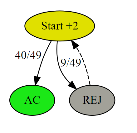
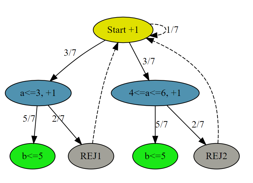
# AC # Runtime: 408 ms, faster than 23.80% of Python3 online submissions for Implement Rand10() Using Rand7(). # Memory Usage: 16.7 MB, less than 90.76% of Python3 online submissions for Implement Rand10() Using Rand7(). classSolution: defrand10(self): whileTrue: a = rand7() if a <= 3: b = rand7() if b <= 5: return b elif a <= 6: b = rand7() if b <= 5: return b + 5
# AC # Runtime: 376 ms, faster than 54.71% of Python3 online submissions for Implement Rand10() Using Rand7(). # Memory Usage: 16.9 MB, less than 38.54% of Python3 online submissions for Implement Rand10() Using Rand7(). classSolution: defrand10(self): whileTrue: a, b = rand7(), rand7() num = (a - 1) * 7 + b if num <= 40: return num % 10 + 1
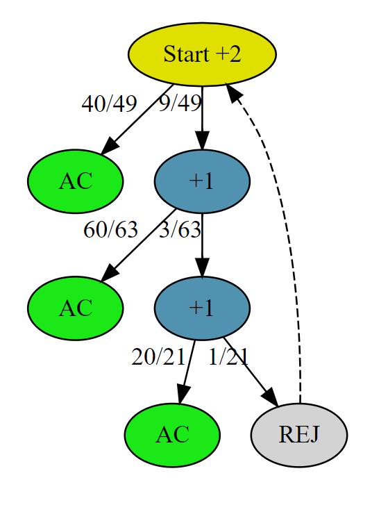
# AC # Runtime: 344 ms, faster than 92.72% of Python3 online submissions for Implement Rand10() Using Rand7(). # Memory Usage: 16.7 MB, less than 90.76% of Python3 online submissions for Implement Rand10() Using Rand7(). classSolution: defrand10(self): whileTrue: a, b = rand7(), rand7() num = (a - 1) * 7 + b if num <= 40: return num % 10 + 1 a = num - 40 b = rand7() num = (a - 1) * 7 + b if num <= 60: return num % 10 + 1 a = num - 60 b = rand7() num = (a - 1) * 7 + b if num <= 20: return num % 10 + 1
# The rand7() API is already defined for you. rand7_c = 0 rand10_c = 0
defrand7(): global rand7_c rand7_c += 1 import random return random.randint(1, 7) defrand10(): global rand10_c rand10_c += 1 whileTrue: a, b = rand7(), rand7() num = (a - 1) * 7 + b if num <= 40: return num % 10 + 1 a = num - 40# [1, 9] b = rand7() num = (a - 1) * 7 + b # [1, 63] if num <= 60: return num % 10 + 1 a = num - 60# [1, 3] b = rand7() num = (a - 1) * 7 + b # [1, 21] if num <= 20: return num % 10 + 1
if __name__ == '__main__': whileTrue: rand10() print(f'{rand10_c}{round(rand7_c/rand10_c, 2)}')
最直接的方式是暴力枚举出所有分组的可能。因为 2N
个人平均分成两组,总数为 \({2n \choose
n}\),是 n 的指数级数量。在文章24
点游戏算法题的 Python 函数式实现: 学用itertools,yield,yield from
巧刷题,我们展示如何调用 Python 的
itertools包,这里,我们也用同样的方式产生 [0, 2N]
的所有集合大小为N的可能(保存在left_set_list中),再遍历找到最小值即可。当然,这种解法会TLE,只是举个例子来体会一下暴力做法。
{linenos
1 2 3 4 5 6 7 8 9 10 11 12 13 14 15 16 17 18
import math from typing importList
classSolution: deftwoCitySchedCost(self, costs: List[List[int]]) -> int: L = range(len(costs)) from itertools import combinations left_set_list = [set(c) for c in combinations(list(L), len(L)//2)]
min_total = math.inf for left_set in left_set_list: cost = 0 for i in L: is_left = 1if i in left_set else0 cost += costs[i][is_left] min_total = min(min_total, cost)
return min_total
O(N) AC解法
对于组合优化问题来说,例如TSP问题(解法链接 TSP问题从DP算法到深度学习1:递归DP方法
AC AIZU TSP问题),一般都是
NP-Hard问题,意味着没有多项次复杂度的解法。但是这个问题比较特殊,它增加了一个特定条件:去城市A和城市B的人数相同,也就是我们已经知道两个分组的数量是一样的。我们仔细思考一下这个意味着什么?考虑只有四个人的小规模情况,如果让你来手动规划,你一定不会穷举出所有两两分组的可能,而是比较人与人相对的两个城市的cost差。举个例子,有如下四个人的costs
# AC # Runtime: 36 ms, faster than 87.77% of Python3 online submissions # Memory Usage: 14.5 MB, less than 14.84% of Python3 online from typing importList
classSolution: deftwoCitySchedCost(self, costs: List[List[int]]) -> int: L = range(len(costs)) cost_diff_lst = [(i, costs[i][0] - costs[i][1]) for i in L] cost_diff_lst.sort(key=lambda x: x[1])
total_cost = 0 for c, (idx, _) inenumerate(cost_diff_lst): is_left = 0if c < len(L) // 2else1 total_cost += costs[idx][is_left]
model = cp_model.CpModel() x = [] total_cost = model.NewIntVar(0, 10000, 'total_cost') for i in I: t = [] for j inrange(2): t.append(model.NewBoolVar('x[%i,%i]' % (i, j))) x.append(t)
# Constraints # Each person must be assigned to at exact one city [model.Add(sum(x[i][j] for j inrange(2)) == 1) for i in I] # equal number of person assigned to two cities model.Add(sum(x[i][0] for i in I) == (len(I) // 2))
# Total cost model.Add(total_cost == sum(x[i][0] * costs[i][0] + x[i][1] * costs[i][1] for i in I)) model.Minimize(total_cost)
solver = cp_model.CpSolver() status = solver.Solve(model)
if status == cp_model.OPTIMAL: print('Total min cost = %i' % solver.ObjectiveValue()) print() for i in I: for j inrange(2): if solver.Value(x[i][j]) == 1: print('People ', i, ' assigned to city ', j, ' Cost = ', costs[i][j])
items=[i for i in I] city_a = pulp.LpVariable.dicts('left', items, 0, 1, pulp.LpBinary) city_b = pulp.LpVariable.dicts('right', items, 0, 1, pulp.LpBinary)
m = pulp.LpProblem("Two Cities", pulp.LpMinimize)
m += pulp.lpSum((costs[i][0] * city_a[i] + costs[i][1] * city_b[i]) for i in items)
# Constraints # Each person must be assigned to at exact one city for i in I: m += pulp.lpSum([city_a[i] + city_b[i]]) == 1 # create a binary variable to state that a table setting is used m += pulp.lpSum(city_a[i] for i in I) == (len(I) // 2)
m.solve()
total = 0 for i in I: if city_a[i].value() == 1.0: total += costs[i][0] else: total += costs[i][1]
# AC # Runtime: 32 ms, faster than 54.28% of Python3 online submissions for Pow(x, n). # Memory Usage: 14.2 MB, less than 5.04% of Python3 online submissions for Pow(x, n).
classSolution: defmyPow(self, x: float, n: int) -> float: ret = 1.0 i = abs(n) while i != 0: if i & 1: ret *= x x *= x i = i >> 1 return1.0 / ret if n < 0else ret
对应的 Java 的代码。
{linenos
1 2 3 4 5 6 7 8 9 10 11 12 13 14 15 16 17 18 19
// AC // Runtime: 1 ms, faster than 42.98% of Java online submissions for Pow(x, n). // Memory Usage: 38.7 MB, less than 48.31% of Java online submissions for Pow(x, n).
classSolution{ publicdoublemyPow(double x, int n){ double ret = 1.0; long i = Math.abs((long) n); while (i != 0) { if ((i & 1) > 0) { ret *= x; } x *= x; i = i >> 1; }
publicint[][] matrixProd(int[][] A, int[][] B) { int R = A.length; int C = B[0].length; int P = A[0].length; int[][] ret = newint[R][C]; for (int r = 0; r < R; r++) { for (int c = 0; c < C; c++) { for (int p = 0; p < P; p++) { ret[r][c] += A[r][p] * B[p][c]; } } } return ret; }
The Fibonacci numbers, commonly denoted F(n) form a
sequence, called the Fibonacci sequence, such that each
number is the sum of the two preceding ones, starting from 0 and 1. That
is,
1 2
F(0) = 0, F(1) = 1 F(N) = F(N - 1) + F(N - 2), for N > 1.
/** * AC * Runtime: 0 ms, faster than 100.00% of Java online submissions for Fibonacci Number. * Memory Usage: 37.9 MB, less than 18.62% of Java online submissions for Fibonacci Number. * * Method: Matrix Fast Power Exponentiation * Time Complexity: O(log(N)) **/ classSolution{ publicintfib(int N){ if (N <= 1) { return N; } int[][] M = {{1, 1}, {1, 0}}; // powers = M^(N-1) N--; int[][] powerDouble = M; int[][] powers = {{1, 0}, {0, 1}}; while (N > 0) { if (N % 2 == 1) { powers = matrixProd(powers, powerDouble); } powerDouble = matrixProd(powerDouble, powerDouble); N = N / 2; }
return powers[0][0]; }
publicint[][] matrixProd(int[][] A, int[][] B) { int R = A.length; int C = B[0].length; int P = A[0].length; int[][] ret = newint[R][C]; for (int r = 0; r < R; r++) { for (int c = 0; c < C; c++) { for (int p = 0; p < P; p++) { ret[r][c] += A[r][p] * B[p][c]; } } } return ret; }
# AC # Runtime: 256 ms, faster than 26.21% of Python3 online submissions for Fibonacci Number. # Memory Usage: 29.4 MB, less than 5.25% of Python3 online submissions for Fibonacci Number.
classSolution:
deffib(self, N: int) -> int: if N <= 1: return N
import numpy as np F = np.array([[1, 1], [1, 0]])
N -= 1 powerDouble = F powers = np.array([[1, 0], [0, 1]]) while N > 0: if N % 2 == 1: powers = np.matmul(powers, powerDouble) powerDouble = np.matmul(powerDouble, powerDouble) N = N // 2
return powers[0][0]
或者也可以直接调用numpy.matrix_power() 代替手动的快速矩阵幂运算。
{linenos
1 2 3 4 5 6 7 8 9 10 11 12 13 14 15 16
# AC # Runtime: 116 ms, faster than 26.25% of Python3 online submissions for Fibonacci Number. # Memory Usage: 29.2 MB, less than 5.25% of Python3 online submissions for Fibonacci Number.
classSolution:
deffib(self, N: int) -> int: if N <= 1: return N
from numpy.linalg import matrix_power import numpy as np F = np.array([[1, 1], [1, 0]]) F = matrix_power(F, N - 1)
return F[0][0]
Leetcode
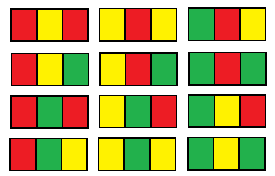
1411. Number of Ways to Paint N × 3 Grid (Hard)
You have a grid of size n x 3 and you want
to paint each cell of the grid with exactly one of the three colours:
Red, Yellow or Green
while making sure that no two adjacent cells have the same colour (i.e
no two cells that share vertical or horizontal sides have the same
colour).
You are given n the number of rows of the grid.
Return the number of ways you can paint this
grid. As the answer may grow large, the answer must
be computed modulo 10^9 + 7.
Example 1:
1 2 3
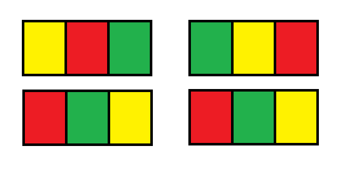
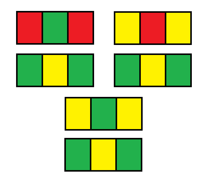
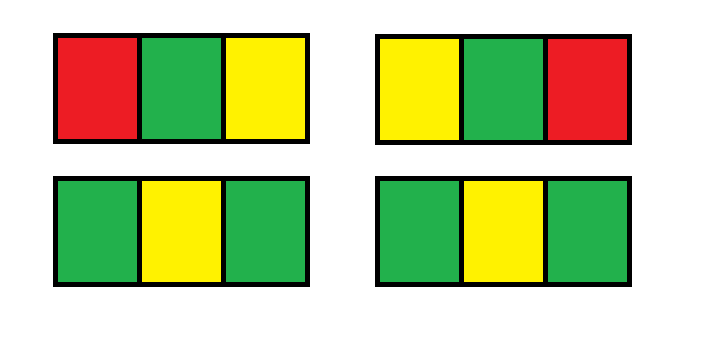
Input: n = 1 Output: 12 Explanation: There are 12 possible way to paint the grid as shown:
# AC # Runtime: 36 ms, faster than 98.88% of Python3 online submissions for Number of Ways to Paint N × 3 Grid. # Memory Usage: 13.9 MB, less than 58.66% of Python3 online submissions for Number of Ways to Paint N × 3 Grid.
classSolution: defnumOfWays(self, n: int) -> int: MOD = 10 ** 9 + 7 dp2, dp3 = 6, 6 n -= 1 while n > 0: dp2, dp3 = (dp2 * 3 + dp3 * 2) % MOD, (dp2 * 2 + dp3 * 2) % MOD n -= 1 return (dp2 + dp3) % MOD
/** AC Runtime: 0 ms, faster than 100.00% of Java online submissions for Number of Ways to Paint N × 3 Grid. Memory Usage: 35.7 MB, less than 97.21% of Java online submissions for Number of Ways to Paint N × 3 Grid. **/
classSolution{ publicintnumOfWays(int n){ long MOD = (long) (1e9 + 7); long[][] ret = {{6, 6}}; long[][] m = {{3, 2}, {2, 2}}; n -= 1; while(n > 0) { if ((n & 1) > 0) { ret = matrixProd(ret, m, MOD); } m = matrixProd(m, m, MOD); n >>= 1; } return (int) ((ret[0][0] + ret[0][1]) % MOD);
}
publiclong[][] matrixProd(long[][] A, long[][] B, long MOD) { int R = A.length; int C = B[0].length; int P = A[0].length; long[][] ret = newlong[R][C]; for (int r = 0; r < R; r++) { for (int c = 0; c < C; c++) { for (int p = 0; p < P; p++) { ret[r][c] += A[r][p] * B[p][c]; ret[r][c] = ret[r][c] % MOD; } } } return ret; }
}
Python 3实现为
{linenos
1 2 3 4 5 6 7 8 9 10 11 12 13 14 15 16 17 18 19
# AC # Runtime: 88 ms, faster than 39.07% of Python3 online submissions for Number of Ways to Paint N × 3 Grid. # Memory Usage: 30.2 MB, less than 11.59% of Python3 online submissions for Number of Ways to Paint N × 3 Grid.
classSolution: defnumOfWays(self, n: int) -> int: import numpy as np
MOD = int(1e9 + 7) ret = np.array([[6, 6]]) m = np.array([[3, 2], [2, 2]])
n -= 1 while n > 0: if n % 2 == 1: ret = np.matmul(ret, m) % MOD m = np.matmul(m, m) % MOD n = n // 2 returnint((ret[0][0] + ret[0][1]) % MOD)
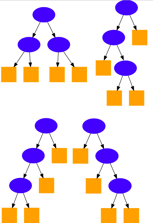
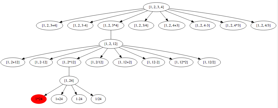
Leetcode 679 24 Game
(Hard) > You have 4 cards each containing a number from 1 to 9.
You need to judge whether they could operated through *, /, +, -, (, )
to get the value of 24.
# AC # Runtime: 36 ms, faster than 91.78% of Python3 online submissions for Permutations. # Memory Usage: 13.9 MB, less than 66.52% of Python3 online submissions for Permutations.
from itertools import permutations from typing importList
classSolution: defpermute(self, nums: List[int]) -> List[List[int]]: return [p for p in permutations(nums)]
# AC # Runtime: 84 ms, faster than 95.43% of Python3 online submissions for Combinations. # Memory Usage: 15.2 MB, less than 68.98% of Python3 online submissions for Combinations. from itertools import combinations from typing importList
classSolution: defcombine(self, n: int, k: int) -> List[List[int]]: return [c for c in combinations(list(range(1, n + 1)), k)]
itertools.product
当有多维度的对象需要迭代笛卡尔积时,可以用 product(iter1, iter2,
...)来生成generator,等价于多重 for 循环。
1 2
[lst for lst in product([1, 2, 3], ['a', 'b'])] [(i, s) for i in [1, 2, 3] for s in ['a', 'b']]
Given a string containing digits from 2-9 inclusive, return all
possible letter combinations that the number could represent. A mapping
of digit to letters (just like on the telephone buttons) is given below.
Note that 1 does not map to any letters.
# AC # Runtime: 24 ms, faster than 94.50% of Python3 online submissions for Letter Combinations of a Phone Number. # Memory Usage: 13.7 MB, less than 83.64% of Python3 online submissions for Letter Combinations of a Phone Number.
from itertools import product from typing importList
classSolution: defletterCombinations(self, digits: str) -> List[str]: if digits == "": return [] mapping = {'2':'abc', '3':'def', '4':'ghi', '5':'jkl', '6':'mno', '7':'pqrs', '8':'tuv', '9':'wxyz'} iter_dims = [mapping[i] for i in digits]
result = [] for lst in product(*iter_dims): result.append(''.join(lst))
The Fibonacci numbers, commonly denoted F(n) form a sequence, called
the Fibonacci sequence, such that each number is the sum of the two
preceding ones, starting from 0 and 1. That is, F(0) = 0, F(1) = 1 F(N)
= F(N - 1) + F(N - 2), for N > 1. Given N, calculate F(N).
# AC # Runtime: 28 ms, faster than 85.56% of Python3 online submissions for Fibonacci Number. # Memory Usage: 13.8 MB, less than 58.41% of Python3 online submissions for Fibonacci Number.
classSolution: deffib(self, N: int) -> int: if N <= 1: return N i = 2 for fib in self.fib_next(): if i == N: return fib i += 1 deffib_next(self): f_last2, f_last = 0, 1 whileTrue: f = f_last2 + f_last f_last2, f_last = f_last, f yield f
yield from 示例
上述yield用法之后,再来演示 yield from 的用法。Yield from 始于Python
3.3,用于嵌套generator时的控制转移,一种典型的用法是有多个generator嵌套时,外层的outer_generator
用 yield from 这种方式等价代替如下代码。
1 2 3
defouter_generator(): for i in inner_generator(): yield i
# AC # Runtime: 48 ms, faster than 90.31% of Python3 online submissions for Kth Smallest Element in a BST. # Memory Usage: 17.9 MB, less than 14.91% of Python3 online submissions for Kth Smallest Element in a BST.
classSolution: defkthSmallest(self, root: TreeNode, k: int) -> int: defordered_iter(node): if node: for sub_node in ordered_iter(node.left): yield sub_node yield node for sub_node in ordered_iter(node.right): yield sub_node
for node in ordered_iter(root): k -= 1 if k == 0: return node.val
等价于如下 yield from 版本:
{linenos
1 2 3 4 5 6 7 8 9 10 11 12 13 14 15 16
# AC # Runtime: 56 ms, faster than 63.74% of Python3 online submissions for Kth Smallest Element in a BST. # Memory Usage: 17.7 MB, less than 73.33% of Python3 online submissions for Kth Smallest Element in a BST.
# AC # Runtime: 112 ms, faster than 57.59% of Python3 online submissions for 24 Game. # Memory Usage: 13.7 MB, less than 85.60% of Python3 online submissions for 24 Game.
import math from itertools import permutations, product from typing importList
defjudgePoint24(self, nums: List[int]) -> bool: mul = lambda x, y: x * y plus = lambda x, y: x + y div = lambda x, y: x / y if y != 0else math.inf minus = lambda x, y: x - y
op_lst = [plus, minus, mul, div]
for ops in product(op_lst, repeat=3): for val in permutations(nums): for v in self.iter_trees(ops[0], ops[1], ops[2], val[0], val[1], val[2], val[3]): ifabs(v - 24) < 0.0001: returnTrue returnFalse
# AC # Runtime: 116 ms, faster than 56.23% of Python3 online submissions for 24 Game. # Memory Usage: 13.9 MB, less than 44.89% of Python3 online submissions for 24 Game.
import math from itertools import combinations, product, permutations from typing importList
classSolution:
defjudgePoint24(self, nums: List[int]) -> bool: mul = lambda x, y: x * y plus = lambda x, y: x + y div = lambda x, y: x / y if y != 0else math.inf minus = lambda x, y: x - y
op_lst = [plus, minus, mul, div]
defrecurse(lst: List[int]): iflen(lst) == 2: for op, values in product(op_lst, permutations(lst)): yield op(values[0], values[1]) else: # choose 2 indices from lst of length n for choosen_idx_lst in combinations(list(range(len(lst))), 2): # remaining indices not choosen (of length n-2) idx_remaining_set = set(list(range(len(lst)))) - set(choosen_idx_lst)
# remaining values not choosen (of length n-2) value_remaining_lst = list(map(lambda x: lst[x], idx_remaining_set)) for op, idx_lst in product(op_lst, permutations(choosen_idx_lst)): # 2 choosen values are lst[idx_lst[0]], lst[idx_lst[1] value_remaining_lst.append(op(lst[idx_lst[0]], lst[idx_lst[1]])) yieldfrom recurse(value_remaining_lst) value_remaining_lst = value_remaining_lst[:-1]
for v in recurse(nums): ifabs(v - 24) < 0.0001: returnTrue
defsimulate_bruteforce(n: int) -> bool: """ Simulates one round. Unbounded time complexity. :param n: total number of seats :return: True if last one has last seat, otherwise False """
seats = [Falsefor _ inrange(n)]
for i inrange(n-1): if i == 0: # first one, always random seats[random.randint(0, n - 1)] = True else: ifnot seats[i]: # i-th has his seat seats[i] = True else: whileTrue: rnd = random.randint(0, n - 1) # random until no conflicts ifnot seats[rnd]: seats[rnd] = True break returnnot seats[n-1]
defsimulate_online(n: int) -> bool: """ Simulates one round of complexity O(N). :param n: total number of seats :return: True if last one has last seat, otherwise False """
# for each person, the seats array idx available are [i, n-1] for i inrange(n-1): if i == 0: # first one, always random rnd = random.randint(0, n - 1) swap(rnd, 0) else: if seats[i] == i: # i-th still has his seat pass else: rnd = random.randint(i, n - 1) # selects idx from [i, n-1] swap(rnd, i) return seats[n-1] == n - 1
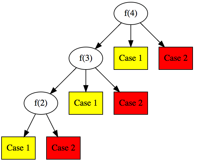
递推思维
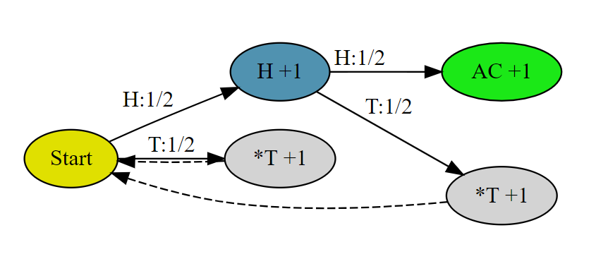
这一节我们用数学递推思维来解释0.5的解。令f(n) 为第 n
位乘客坐在自己的座位上的概率,考察第一个人的情况(first step
analysis),有三种可能
这种思想可以写出如下代码,seats为 n 大小的bool
数组,当第i个人(0<i<n)发现自己座位被占的话,此时必然seats[0]没有被占,同时seats[i+1:]都是空的。假设seats[0]被占的话,要么是第一个人占的,要么是第p个人(p<i)坐了,两种情况下乱序都已经恢复了,此时第i个座位一定是空的。
defsimulate(n: int) -> bool: """ Simulates one round of complexity O(N). :param n: total number of seats :return: True if last one has last seat, otherwise False """
seats = [Falsefor _ inrange(n)]
for i inrange(n-1): if i == 0: # first one, always random rnd = random.randint(0, n - 1) seats[rnd] = True else: ifnot seats[i]: # i-th still has his seat seats[i] = True else: # 0 must not be available, now we have 0 and [i+1, n-1], rnd = random.randint(i, n - 1) if rnd == i: seats[0] = True else: seats[rnd] = True returnnot seats[n-1]


.png)
.png)