#OpenAI Gym

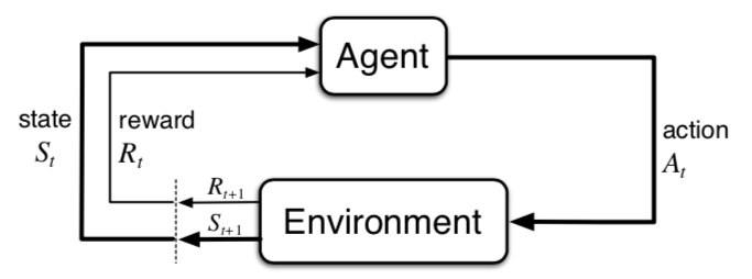
这一期我们进入第六章:时序差分学习(Temporal-Difference Learning)。TD Learning本质上是加了bootstrapping的蒙特卡洛(MC),也是model-free的方法,但实践中往往比蒙特卡洛收敛更快。我们选取OpenAI Gym中经典的CartPole环境来讲解TD。更多相关内容,欢迎关注 本公众号 MyEncyclopedia

CartPole OpenAI 环境

如图所示,小车上放了一根杆,杆会根据物理系统定理因重力而倒下,我们可以控制小车往左或者往右,目的是尽可能地让杆保持树立状态。

CartPole OpenAI Gym

CartPole 观察到的状态是四维的float值,分别是车位置,车速度,杆角度和杆角速度。下表为四个维度的值范围。给到小车的动作,即action space,只有两种:0,表示往左推;1,表示往右推。

Min Max
Cart Position -4.8 4.8
Cart Velocity -Inf Inf
Pole Angle -0.418 rad (-24 deg) 0.418 rad (24 deg)
Pole Angular Velocity -Inf Inf

离散化连续状态

从上所知,CartPole step() 函数返回了4维ndarray,类型为float32的连续状态空间。对于传统的tabular方法来说第一步必须离散化状态,目的是可以作为Q table的主键来查找。下面定义的State类型是离散化后的具体类型,另外 Action 类型已经是0和1,不需要做离散化处理。

{linenos
1
2
State = Tuple[int, int, int, int]
Action = int

离散化处理时需要考虑的一个问题是如何设置每个维度的分桶策略。分桶策略会决定性地影响训练的效果。原则上必须将和action以及reward强相关的维度做细粒度分桶,弱相关或者无关的维度做粗粒度分桶。举个例子,小车位置本身并不能影响Agent采取的下一动作,当给定其他三维状态的前提下,因此我们对小车位置这一维度仅设置一个桶(bucket size=1)。而杆的角度和角速度是决定下一动作的关键因素,因此我们分别设置成6个和12个。

以下是离散化相关代码,四个维度的 buckets=(1, 2, 6, 12)。self.q是action value的查找表,具体类型是shape 为 (1, 2, 6, 12, 2) 的ndarray。

{linenos
1
2
3
4
5
6
7
8
9
10
11
12
13
14
15
16
17
18
19
20
21
class CartPoleAbstractAgent(metaclass=abc.ABCMeta):
def __init__(self, buckets=(1, 2, 6, 12), discount=0.98, lr_min=0.1, epsilon_min=0.1):
self.env = gym.make('CartPole-v0')

env = self.env
# [position, velocity, angle, angular velocity]
self.dims_config = [(env.observation_space.low[0], env.observation_space.high[0], 1),
(-0.5, 0.5, 1),
(env.observation_space.low[2], env.observation_space.high[2], 6),
(-math.radians(50) / 1., math.radians(50) / 1., 12)]
self.q = np.zeros(buckets + (self.env.action_space.n,))
self.pi = np.zeros_like(self.q)
self.pi[:] = 1.0 / env.action_space.n

def to_bin_idx(self, val: float, lower: float, upper: float, bucket_num: int) -> int:
percent = (val + abs(lower)) / (upper - lower)
return min(bucket_num - 1, max(0, int(round((bucket_num - 1) * percent))))

def discretize(self, obs: np.ndarray) -> State:
discrete_states = tuple([self.to_bin_idx(obs[d], *self.dims_config[d]) for d in range(len(obs))])
return discrete_states

train() 方法串联起来 agent 和 env 交互的流程,包括从 env 得到连续状态转换成离散状态,更新 Agent 的 Q table 甚至 Agent的执行policy,choose_action会根据执行 policy 选取action。

{linenos
1
2
3
4
5
6
7
8
9
10
11
12
13
14
15
16
def train(self, num_episodes=2000):
for e in range(num_episodes):
print(e)
s: State = self.discretize(self.env.reset())

self.adjust_learning_rate(e)
self.adjust_epsilon(e)
done = False

while not done:
action: Action = self.choose_action(s)
obs, reward, done, _ = self.env.step(action)
s_next: State = self.discretize(obs)
a_next = self.choose_action(s_next)
self.update_q(s, action, reward, s_next, a_next)
s = s_next

choose_action 的默认实现为基于现有 Q table 的 \(\epsilon\)-greedy 策略。

{linenos
1
2
3
4
5
def choose_action(self, state) -> Action:
if np.random.random() < self.epsilon:
return self.env.action_space.sample()
else:
return np.argmax(self.q[state])

抽象出公共的基类代码 CartPoleAbstractAgent 之后,SARSA、Q-Learning和Expected SARSA只需要复写 update_q 抽象方法即可。

{linenos
1
2
3
4
class CartPoleAbstractAgent(metaclass=abc.ABCMeta):
@abc.abstractmethod
def update_q(self, s: State, a: Action, r, s_next: State, a_next: Action):
pass

TD Learning的精髓

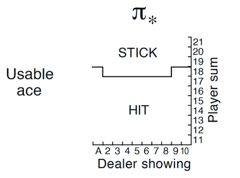
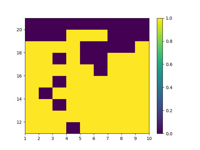
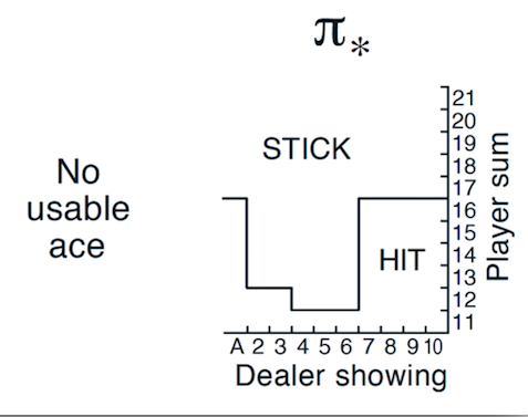
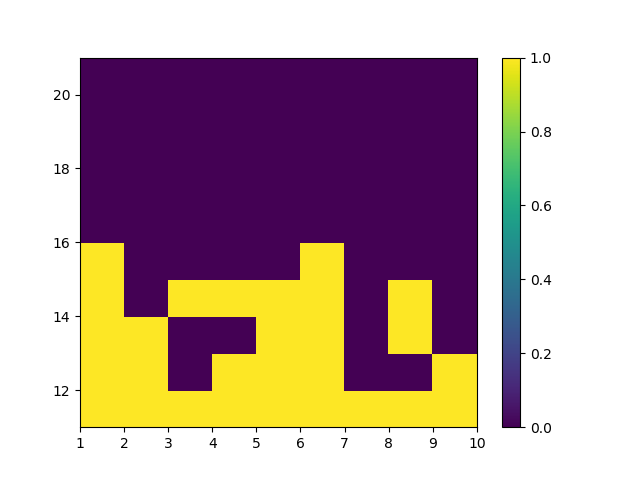
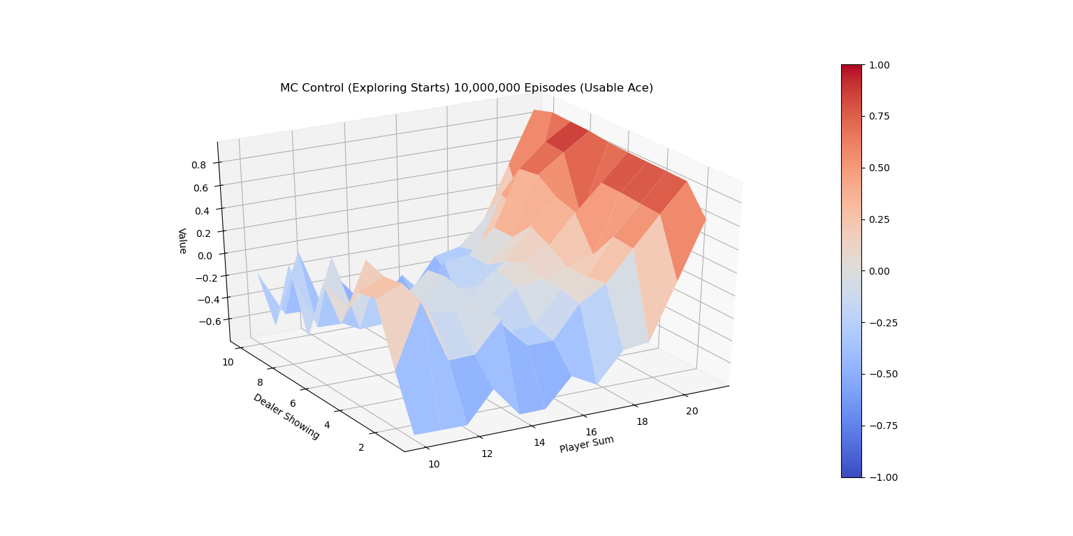
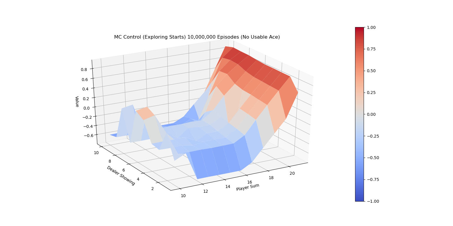
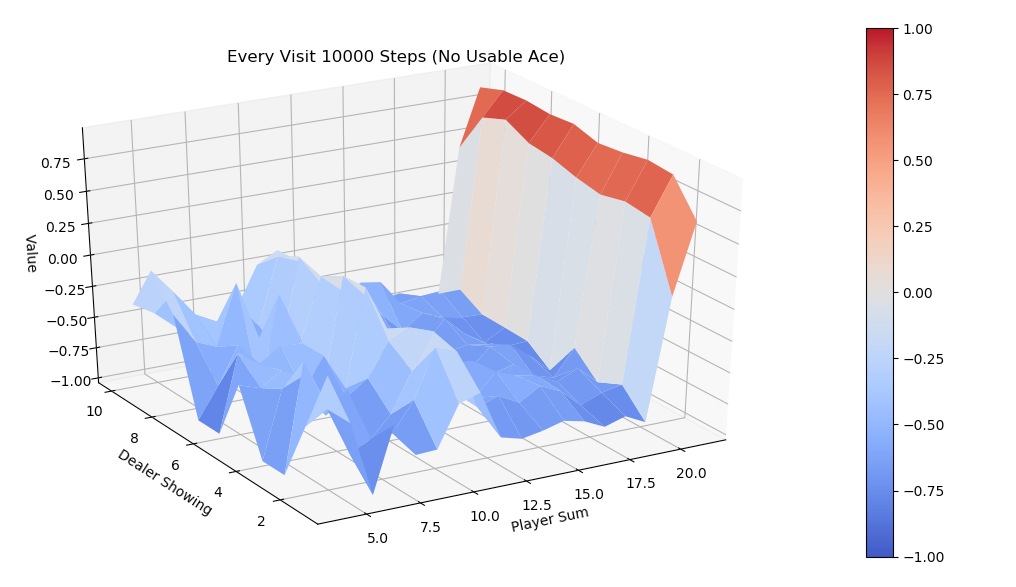
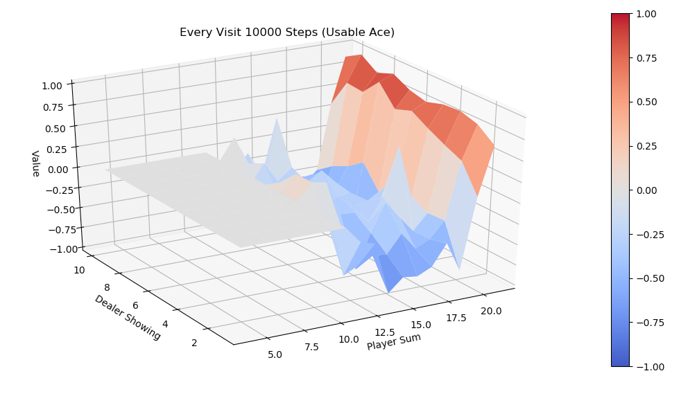
在上一期,本公众号 MyEncyclopedia 的21点游戏的蒙特卡洛On-Policy控制介绍了Monte Carlo方法,知道MC需要在环境中模拟直至最终结局。若记\(G_t\)为t步以后的最终return,则 MC online update 版本更新为:

\[ V(S_t) \leftarrow V(S_t) + \alpha[G_{t} - V(S_t)] \]

可以认为 \(V(S_t)\) 向着目标为 \(G_t\) 更新了一小步。

而TD方法可以只模拟下一步,得到 \(R_{t+1}\),而余下步骤的return,\(G_t - R_{t+1}\) 用已有的 \(V(S_{t+1})\) 来估计,或者统计上称作bootstrapping。这样 TD 的更新目标值变成 \(R_{t+1} + \gamma V(S_{t+1})\),整体online update 公式则为: \[ V(S_t) \leftarrow V(S_t) + \alpha[R_{t+1} + \gamma V(S_{t+1})- V(S_t)] \]

概念上,如果只使用下一步 \(R_{t+1}\) 值然后bootstrap称为 TD(0),用于区分使用多步后的reward的TD方法。另外,变化的数值 \(R_{t+1} + \gamma V(S_{t+1})- V(S_t)\) 称为TD error。

另外一个和Monte Carlo的区别在于一般TD方法保存更精细的Q值,\(Q(S_t, A_t)\),并用Q值来boostrap,而MC一般用V值也可用Q值。

SARSA: On-policy TD 控制

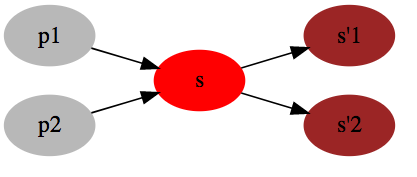
SARSA的命名源于一次迭代产生了五元组 \(S_t,A_t,R_{t+1},S_{t+1},A_{t+1}\)。SARSA利用五个值做 action-value的 online update:

\[ Q(S_t,A_t) \leftarrow Q(S_t,A_t) + \alpha[R_{t+1}+\gamma Q(S_{t+1}, A_{t+1}) - Q(S_t,A_t)] \]

对应的Q table更新实现为:

{linenos
1
2
3
4
class SarsaAgent(CartPoleAbstractAgent):

def update_q(self, s: State, a: Action, r, s_next: State, a_next: Action):
self.q[s][a] += self.lr * (r + self.discount * (self.q[s_next][a_next]) - self.q[s][a])

SARSA 在执行policy 后的Q值更新是对于针对于同一个policy的,完成了一次策略迭代(policy iteration),这个特点区分于后面的Q-learning算法,这也是SARSA 被称为 On-policy 的原因。下面是完整算法伪代码。

\[ \begin{align*} &\textbf{Sarsa (on-policy TD Control) for estimating } Q \approx q_{*} \\ & \text{Algorithm parameters: step size }\alpha \in ({0,1}]\text{, small }\epsilon > 0 \\ & \text{Initialize }Q(s,a), \text{for all } s \in \mathcal{S}^{+}, a \in \mathcal{A}(s) \text{, arbitrarily except that } Q(terminal, \cdot) = 0 \\ & \text{Loop for each episode:}\\ & \quad \text{Initialize }S\\ & \quad \text{Choose } A \text{ from } S \text{ using policy derived from } Q \text{ (e.g., } \epsilon\text{-greedy)} \\ & \quad \text{Loop for each step of episode:} \\ & \quad \quad \text{Take action }A, \text { observe } R, S^{\prime} \\ & \quad \quad \text{Choose }A^{\prime} \text { from } S^{\prime} \text{ using policy derived from } Q \text{ (e.g., } \epsilon\text{-greedy)} \\ & \quad \quad Q(S,A) \leftarrow Q(S,A) + \alpha[R+\gamma Q(S^{\prime}, A^{\prime}) - Q(S,A)] \\ & \quad \quad S \leftarrow S^{\prime}; A \leftarrow A^{\prime} \\ & \quad \text{until }S\text{ is terminal} \\ \end{align*} \]

SARSA 训练分析

SARSA收敛较慢,1000次episode后还无法持久稳定,后面的Q-learning 和 Expected Sarsa 都可以在1000次episode学习长时间保持不倒的状态。

Q-Learning: Off-policy TD 控制

Q-Learning 是深度学习时代前强化学习领域中的著名算法,它的 online update 公式为: \[ Q(S_t,A_t) \leftarrow Q(S_t,A_t) + \alpha[R_{t+1}+\gamma \max_{a}Q(S_{t+1}, a) - Q(S_t,A_t)] \]

对应的 update_q() 方法具体实现

{linenos
1
2
3
4
class QLearningAgent(CartPoleAbstractAgent):

def update_q(self, s: State, a: Action, r, s_next: State, a_next: Action):
self.q[s][a] += self.lr * (r + self.discount * np.max(self.q[s_next]) - self.q[s][a])

本质上用现有的Q table中最好的action来bootrap 对应的最佳Q值,推导如下:

\[ \begin{aligned} q_{*}(s, a) &=\mathbb{E}\left[R_{t+1}+\gamma \max _{a^{\prime}} q_{*}\left(S_{t+1}, a^{\prime}\right) \mid S_{t}=s, A_{t}=a\right] \\ &=\mathbb{E}[R \mid S_{t}=s, A_{t}=a] + \gamma\sum_{s^{\prime}} p\left(s^{\prime}\mid s, a\right)\max _{a^{\prime}} q_{*}\left(s^{\prime}, a^{\prime}\right) \\ &\approx r + \gamma \max _{a^{\prime}} q_{*}\left(s^{\prime}, a^{\prime}\right) \end{aligned} \]

Q-Learning 被称为 off-policy 的原因是它并没有完成一次policy iteration,而是直接用已有的 Q 来不断近似 \(Q_{*}\)

对比下面的Q-Learning 伪代码和之前的 SARSA 版本可以发现,Q-Learning少了一次模拟后的 \(A_{t+1}\),这也是Q-Learning 中执行policy和预估Q值(即off-policy)分离的一个特征。

\[ \begin{align*} &\textbf{Q-learning (off-policy TD Control) for estimating } \pi \approx \pi_{*} \\ & \text{Algorithm parameters: step size }\alpha \in ({0,1}]\text{, small }\epsilon > 0 \\ & \text{Initialize }Q(s,a), \text{for all } s \in \mathcal{S}^{+}, a \in \mathcal{A}(s) \text{, arbitrarily except that } Q(terminal, \cdot) = 0 \\ & \text{Loop for each episode:}\\ & \quad \text{Initialize }S\\ & \quad \text{Loop for each step of episode:} \\ & \quad \quad \text{Choose } A \text{ from } S \text{ using policy derived from } Q \text{ (e.g., } \epsilon\text{-greedy)} \\ & \quad \quad \text{Take action }A, \text { observe } R, S^{\prime} \\ & \quad \quad Q(S,A) \leftarrow Q(S,A) + \alpha[R+\gamma \max_{a}Q(S^{\prime}, a) - Q(S,A)] \\ & \quad \quad S \leftarrow S^{\prime}\\ & \quad \text{until }S\text{ is terminal} \\ \end{align*} \]

Q-Learning 训练分析

Q-Learning 1000次episode就可以持久稳定住。

SARSA 改进版 Expected SARSA

Expected SARSA 改进了 SARSA 的地方在于考虑到了在某一状态下的现有策略动作分布,以此来减少variance,加快收敛,具体更新规则为:

\[ \begin{aligned} Q(S_t,A_t) &\leftarrow Q(S_t,A_t) + \alpha[R_{t+1}+\gamma \mathbb{E}_{\pi}[Q(S_{t+1}, A_{t+1} \mid S_{t+1})] - Q(S_t,A_t)] \\ &\leftarrow Q(S_t,A_t) + \alpha[R_{t+1}+\gamma \sum_{a} \pi\left(a\mid S_{t+1}\right) Q(S_{t+1}, a) - Q(S_t,A_t)] \\ \end{aligned} \]

注意在实现中,update_q() 不仅更新了Q table,还显示更新了执行policy \(\pi\)

{linenos
1
2
3
4
5
6
7
8
9
class ExpectedSarsaAgent(CartPoleAbstractAgent):

def update_q(self, s: State, a: Action, r, s_next: State, a_next: Action):
self.q[s][a] = self.q[s][a] + self.lr * (r + self.discount * np.dot(self.pi[s_next], self.q[s_next]) - self.q[s][a])
# update pi[s]
best_a = np.random.choice(np.where(self.q[s] == max(self.q[s]))[0])
n_actions = self.env.action_space.n
self.pi[s][:] = self.epsilon / n_actions
self.pi[s][best_a] = 1 - (n_actions - 1) * (self.epsilon / n_actions)

同样的,Expected SARSA 1000次迭代也能比较好的学到最佳policy。

这期继续Sutton强化学习第二版,第五章蒙特卡洛方法。在上期21点游戏的策略蒙特卡洛值预测学习了如何用Monte Carlo来预估给定策略 \(\pi\)\(V_{\pi}\) 值之后,这一期我们用Monte Carlo方法来解得21点游戏最佳策略 \(\pi_{*}\)

蒙特卡洛策略提升

回顾一下,在Grid World 策略迭代和值迭代中由于存在Policy Improvement Theorem,我们可以利用环境dynamics信息计算出策略v值,再选取最greedy action的方式改进策略,形成策略提示最终能够不断逼近最佳策略。 \[ \pi_{0} \stackrel{\mathrm{E}}{\longrightarrow} v_{\pi_{0}} \stackrel{\mathrm{I}}{\longrightarrow} \pi_{1} \stackrel{\mathrm{E}}{\longrightarrow} v_{\pi_{1}} \stackrel{\mathrm{I}}{\longrightarrow} \pi_{2} \stackrel{\mathrm{E}}{\longrightarrow} \cdots \stackrel{\mathrm{I}}{\longrightarrow} \pi_{*} \stackrel{\mathrm{E}}{\longrightarrow} v_{*} \] Monte Carlo Control方法搜寻最佳策略 \(\pi{*}\),是否也能沿用同样的思路呢?答案是可行的。不过,不同于第四章中我们已知环境MDP就知道状态的前后依赖关系,进而从v值中能推断出策略 \(\pi\),在Monte Carlo方法中,环境MDP是未知的,因而我们只能从action-value中下手,通过海量Monte Carlo试验来近似 \(q_{\pi}\)。有了策略 Q 值,再和MDP策略迭代方法一样,选取最greedy action的策略,这种策略提示方式理论上被证明了最终能够不断逼近最佳策略。 \[ \pi_{0} \stackrel{\mathrm{E}}{\longrightarrow} q_{\pi_{0}} \stackrel{\mathrm{I}}{\longrightarrow} \pi_{1} \stackrel{\mathrm{E}}{\longrightarrow} q_{\pi_{1}} \stackrel{\mathrm{I}}{\longrightarrow} \pi_{2} \stackrel{\mathrm{E}}{\longrightarrow} \cdots \stackrel{\mathrm{I}}{\longrightarrow} \pi_{*} \stackrel{\mathrm{E}}{\longrightarrow} q_{*} \]

但是此方法有一个前提要满足,由于数据是依据策略 \(\pi_{i}\) 生成的,理论上需要保证在无限次的模拟过程中,每个状态都必须被无限次访问到,才能保证最终每个状态的Q估值收敛到真实的 \(q_{*}\)。满足这个前提的一个简单实现是强制随机环境初始状态,保证每个状态都能有一定概率被生成。这个思路就是 Monte Carlo Control with Exploring Starts算法,伪代码如下:

\[ \begin{align*} &\textbf{Monte Carlo ES (Exploring Starts), for estimating } \pi \approx \pi_{*} \\ & \text{Initialize:} \\ & \quad \pi(s) \in \mathcal A(s) \text{ arbitrarily for all }s \in \mathcal{S} \\ & \quad Q(s, a) \in \mathbb R \text{, arbitrarily, for all }s \in \mathcal{S}, a \in \mathcal A(s) \\ & \quad Returns(s, a) \leftarrow \text{ an empty list, for all }s \in \mathcal{S}, a \in \mathcal A(s)\\ & \\ & \text{Loop forever (for episode):}\\ & \quad \text{Choose } S_0\in \mathcal{S}, A_0 \in \mathcal A(S_0) \text{ randomly such that all pairs have probability > 0} \\ & \quad \text{Generate an episode from } S_0, A_0 \text{, following } \pi : S_0, A_0, R_1, S_1, A_1, R_2, ..., S_{T-1}, A_{T-1}, R_T\\ & \quad G \leftarrow 0\\ & \quad \text{Loop for each step of episode, } t = T-1, T-2, ..., 0:\\ & \quad \quad \quad G \leftarrow \gamma G + R_{t+1}\\ & \quad \quad \quad \text{Unless the pair } S_t, A_t \text{ appears in } S_0, A_0, S_1, A_1, ..., S_{t-1}, A_{t-1}\\ & \quad \quad \quad \quad \text{Append } G \text { to }Returns(S_t, A_t) \\ & \quad \quad \quad \quad Q(S_t, A_t) \leftarrow \operatorname{average}(Returns(S_t, A_t))\\ & \quad \quad \quad \quad \pi(S_t) \leftarrow \operatorname{argmax}_a Q(S_t, a)\\ \end{align*} \]

下面我们实现21点游戏的Monte Carlo ES 算法。21点游戏只有200个有效的状态,可以满足算法要求的生成episode前先随机选择某一状态的前提条件。

相对于上一篇,我们增加 ActionValue和Policy的类型定义,ActionValue表示 \(q(s, a)\) ,是一个State到动作分布的Dict,Policy 类型也一样。Actions为一维ndarray,维数是离散动作数量。

{linenos
1
2
3
4
5
6
State = Tuple[int, int, bool]
Action = bool
Reward = float
Actions = np.ndarray
ActionValue = Dict[State, Actions]
Policy = Dict[State, Actions]

下面代码示例如何给定 Policy后,依据指定状态state的动作分布采样,决定下一动作。

1
2
3
policy: Policy
A: ActionValue = policy[state]
action = np.random.choice([0, 1], p=A/sum(A))

整个算法的 python 代码实现如下:

{linenos
1
2
3
4
5
6
7
8
9
10
11
12
13
14
15
16
17
18
19
20
21
22
23
24
25
26
def mc_control_exploring_starts(env: BlackjackEnv, num_episodes, discount_factor=1.0) \
-> Tuple[ActionValue, Policy]:
states = list(product(range(10, 22), range(1, 11), (True, False)))
policy = {s: np.ones(env.action_space.n) * 1.0 / env.action_space.n for s in states}
Q = defaultdict(lambda: np.zeros(env.action_space.n))
returns_sum = defaultdict(float)
returns_count = defaultdict(float)

for episode_i in range(1, num_episodes + 1):
s0 = random.choice(states)
reset_env_with_s0(env, s0)
episode_history = gen_custom_s0_stochastic_episode(policy, env, s0)

G = 0
for t in range(len(episode_history) - 1, -1, -1):
s, a, r = episode_history[t]
G = discount_factor * G + r
if not any(s_a_r[0] == s and s_a_r[1] == a for s_a_r in episode_history[0: t]):
returns_sum[s, a] += G
returns_count[s, a] += 1.0
Q[s][a] = returns_sum[s, a] / returns_count[s, a]
best_a = np.argmax(Q[s])
policy[s][best_a] = 1.0
policy[s][1-best_a] = 0.0

return Q, policy

在MC Exploring Starts 算法中,我们需要指定环境初始状态,一种做法是env.reset()时接受初始状态,但是考虑到不去修改第三方实现的 BlackjackEnv类,采用一个取巧的办法,在调用reset()后直接改写env 的私有变量,这个逻辑封装在 reset_env_with_s0 方法中。

{linenos
1
2
3
4
5
6
7
8
9
10
11
12
13
14
15
16
17
18
def reset_env_with_s0(env: BlackjackEnv, s0: State) -> BlackjackEnv:
env.reset()
player_sum = s0[0]
oppo_sum = s0[1]
has_usable = s0[2]

env.dealer[0] = oppo_sum
if has_usable:
env.player[0] = 1
env.player[1] = player_sum - 11
else:
if player_sum > 11:
env.player[0] = 10
env.player[1] = player_sum - 10
else:
env.player[0] = 2
env.player[1] = player_sum - 2
return env

算法结果的可视化和理论对比

下图是有Usable Ace情况下的理论最优策略。
理论最佳策略(有Ace)
Monte Carlo方法策略提示的收敛是比较慢的,下图是运行10,000,000次episode后有Usable Ace时的策略 \(\pi_{*}^{\prime}\)。对比理论最优策略,MC ES在不少的状态下还未收敛到理论最优解。
MC ES 10M的最佳策略(有Ace)
同样的,下两张图是无Usable Ace情况下的理论最优策略和试验结果的对比。
理论最佳策略(无Ace)
MC ES 10M的最佳策略(无Ace)
下面的两张图画出了运行代码10,000,000次episode后 \(\pi{*}\)的V值图。
MC ES 10M的最佳V值(有Ace)
MC ES 10M的最佳V值(无Ace)

Exploring Starts 蒙特卡洛控制改进

为了避免Monte Carlo ES Control在初始时必须访问到任意状态的限制,教材中介绍了一种改进算法,On-policy first-visit MC control for \(\epsilon \text{-soft policies}\) ,它同样基于Monte Carlo 预估Q值,但用 \(\epsilon \text{-soft}\) 策略来代替最有可能的action策略作为下一次迭代策略,\(\epsilon \text{-soft}\) 本质上来说就是对于任意动作都保留 \(\epsilon\) 小概率的访问可能,权衡了exploration和exploitation,由于每个动作都可能被无限次访问到,Explorting Starts中的强制随机初始状态就可以去除了。Monte Carlo ES Control 和 On-policy first-visit MC control for \(\epsilon \text{-soft policies}\) 都属于on-policy算法,其区别于off-policy的本质在于预估 \(q_{\pi}(s,a)\)时是否从同策略\(\pi\)生成的数据来计算。一个比较subtle的例子是著名的Q-Learning,因为根据这个定义,Q-Learning属于off-policy。

\[ \begin{align*} &\textbf{On-policy first-visit MC control (for }\epsilon \textbf{-soft policies), estimating } \pi \approx \pi_{*} \\ & \text{Algorithm parameter: small } \epsilon > 0 \\ & \text{Initialize:} \\ & \quad \pi \leftarrow \text{ an arbitrary } \epsilon \text{-soft policy} \\ & \quad Q(s, a) \in \mathbb R \text{, arbitrarily, for all }s \in \mathcal{S}, a \in \mathcal A(s) \\ & \quad Returns(s, a) \leftarrow \text{ an empty list, for all }s \in \mathcal{S}, a \in \mathcal A(s)\\ & \\ & \text{Repeat forever (for episode):}\\ & \quad \text{Generate an episode following } \pi : S_0, A_0, R_1, S_1, A_1, R_2, ..., S_{T-1}, A_{T-1}, R_T\\ & \quad G \leftarrow 0\\ & \quad \text{Loop for each step of episode, } t = T-1, T-2, ..., 0:\\ & \quad \quad \quad G \leftarrow \gamma G + R_{t+1}\\ & \quad \quad \quad \text{Unless the pair } S_t, A_t \text{ appears in } S_0, A_0, S_1, A_1, ..., S_{t-1}, A_{t-1}\\ & \quad \quad \quad \quad \text{Append } G \text { to }Returns(S_t, A_t) \\ & \quad \quad \quad \quad Q(S_t, A_t) \leftarrow \operatorname{average}(Returns(S_t, A_t))\\ & \quad \quad \quad \quad A^{*} \leftarrow \operatorname{argmax}_a Q(S_t, a)\\ & \quad \quad \quad \quad \text{For all } a \in \mathcal A(S_t):\\ & \quad \quad \quad \quad \quad \pi(a|S_t) \leftarrow \begin{cases} 1 - \epsilon + \epsilon / |\mathcal A(S_t)| & \text{ if } a = A^{*}\\ \epsilon / |\mathcal A(S_t)| & \text{ if } a \neq A^{*}\\ \end{cases} \\ \end{align*} \]

伪代码对应的 Python 实现如下。

{linenos
1
2
3
4
5
6
7
8
9
10
11
12
13
14
15
16
17
18
19
20
21
22
23
24
25
26
27
28
def mc_control_epsilon_greedy(env: BlackjackEnv, num_episodes, discount_factor=1.0, epsilon=0.1) \
-> Tuple[ActionValue, Policy]:
returns_sum = defaultdict(float)
returns_count = defaultdict(float)

states = list(product(range(10, 22), range(1, 11), (True, False)))
policy = {s: np.ones(env.action_space.n) * 1.0 / env.action_space.n for s in states}
Q = defaultdict(lambda: np.zeros(env.action_space.n))

def update_epsilon_greedy_policy(policy: Policy, Q: ActionValue, s: State):
policy[s] = np.ones(env.action_space.n, dtype=float) * epsilon / env.action_space.n
best_action = np.argmax(Q[s])
policy[s][best_action] += (1.0 - epsilon)

for episode_i in range(1, num_episodes + 1):
episode_history = gen_stochastic_episode(policy, env)

G = 0
for t in range(len(episode_history) - 1, -1, -1):
s, a, r = episode_history[t]
G = discount_factor * G + r
if not any(s_a_r[0] == s and s_a_r[1] == a for s_a_r in episode_history[0: t]):
returns_sum[s, a] += G
returns_count[s, a] += 1.0
Q[s][a] = returns_sum[s, a] / returns_count[s, a]
update_epsilon_greedy_policy(policy, Q, s)

return Q, policy

从这期开始我们进入Sutton强化学习第二版,第五章蒙特卡洛方法。蒙特卡洛方法是一种在工程各领域都存在的基本方法,在强化领域中,其特点是无需知道环境的dynamics,只需不断模拟记录并分析数据即可逼近理论真实值。蒙特卡洛方法本篇将会用21点游戏作为示例来具体讲解其原理和代码实现。

21点游戏问题

21点游戏是一个经典的赌博游戏。大致规则是玩家和庄家各发两张牌,一张明牌,一张暗牌。玩家和庄家可以决定加牌或停止加牌,新加的牌均为暗牌,最后比较两个玩家的牌面和,更接近21点的获胜。游戏的变化因素是牌Ace,既可以作为11也可以作为1来计算,算作11的时候称作usable。

Sutton教材中的21点游戏规则简化了几个方面用于控制问题状态数:

  • 已发的牌的无状态性:和一副牌的21点游戏不同的是,游戏环境简化为牌是可以无穷尽被补充的,一副牌的某一张被派发后,同样的牌会被补充进来,或者可以认为每次发放的牌都是从一副新牌中抽出的。统计学中的术语称为重复采样(sample with replacement)。这种规则下极端情况下,玩家可以拥有 5个A或者5个2。另外,这会导致玩家无法通过开局看到的3张牌的信息推断后续发牌的概率,如此就大规模减小了游戏状态数。
  • 庄家和玩家独立游戏,无需按轮次要牌。开局给定4张牌后,玩家先行动,加牌直至超21点或者停止要牌,如果超21点,玩家输,否则,等待庄家行动,庄家加牌直至超21点或者停止要牌,如果超21点,庄家输,否则比较两者的总点数。这种方式可以认为当玩家和庄家看到初始的三张牌后独立做一系列决策,最后比较结果,避免了交互模式下因为能观察到每一轮后对方牌数变化产生额外的信息而导致的游戏状态数爆炸。

有以上两个规则的简化,21点游戏问题的总状态数有下面三个维度

  • 自己手中的点数和(12到21)

  • 庄家明牌的点数(A到10)

  • 庄家明牌是否有 A(True, False)。

状态总计总数为三个维度的乘积 10 * 10 * 2 = 200。

关于游戏状态有几个比较subtle的假设或者要素。首先,玩家初始时能看到三张牌,这三张牌确定了状态的三个维度的值,当然也就确定了Agent的初始状态,随后按照独立游戏的规则进行,玩家根据初始状态依照某种策略决策要牌还是结束要牌,新拿的牌更新了游戏状态,玩家转移到新状态下继续做决策。举个例子,假设初始时玩家明牌为8,暗牌为6,庄家明牌为7,则游戏状态为Tuple (14, 7, False)。若玩家的策略为教材中的固定规则策略:没到20或者21继续要牌。下一步玩家拿到牌3,则此时新状态为 (17, 7, False),按照策略继续要牌。

第二个方面是游戏的状态完全等价于玩家观察到的信息。比如尽管初始时有4张牌,真正的状态是这四张牌的值,但是出于简化目的,不考虑partially observable 的情况,即不将暗牌纳入游戏状态中。另外,庄家做决策的时候也无法得知玩家的手中的总牌数。

第三个方面是关于玩家点数。考虑玩家初始时的两张牌为2,3,总点数是5,那么为何不将5加入到游戏状态中呢?原则上是可以将初始总和为2到11都加入到游戏状态,但是意义不大,原因在于我们已经假设了已发牌的无状态性,拿到的这两张牌并不会改变后续补充的牌的出现概率。当玩家初始总和为2到11时一定会追加牌,因为无论第三张牌是什么,都不会超过21点,只会增加获胜概率。若后续第三张牌为8,总和变成13,就进入了有效的游戏状态,因为此时如果继续要牌,获得10,则游戏输掉。因此,我们关心的游戏状态并不完全等价于所有可能的游戏状态。

21点游戏 OpenAI Gym环境

OpenAI Gym 已经实现了Sutton版本的21点游戏环境,并按上述规则来进行。在安装完OpenAI Gym包之后 import BlackjackEnv即可使用。

1
from gym.envs.toy_text import BlackjackEnv

根据这个游戏环境,我们先来定义一些类型,可以令代码更具可读性和抽象化。State 上文说过是由三个分量组成的Tuple。Action 为bool类型 表示是否继续要牌。Reward 为+1或者-1,玩家叫牌过程中为0。StateValue 为书中的 \(V_{\pi}\),实现上是一个Dict。DeterministicPolicy 为一个函数,输入是某一状态,输出是唯一的决策动作。

{linenos
1
2
3
4
5
State = Tuple[int, int, bool]
Action = bool
Reward = float
StateValue = Dict[State, float]
DeterministicPolicy = Callable[[State], Action]

以下代码是 BlackjackEnv 核心代码,step 方法的输入为玩家的决策动作(叫牌还是结束),并输出State, Reward, is_done。简单解释一下代码逻辑,当玩家继续加牌时,需要判断是否超21点,如果没有超过的话,返回下一状态,同时reward 为0,等待下一step方法。若玩家停止叫牌,则按照庄家策略:小于17时叫牌。游戏终局时产生+1表示玩家获胜,-1表示庄家获胜。

{linenos
1
2
3
4
5
6
7
8
9
10
11
12
13
14
15
16
17
18
19
20
21
22
23
class BlackjackEnv(gym.Env):

def step(self, action):
assert self.action_space.contains(action)
if action: # hit: add a card to players hand and return
self.player.append(draw_card(self.np_random))
if is_bust(self.player):
done = True
reward = -1.
else:
done = False
reward = 0.
else: # stick: play out the dealers hand, and score
done = True
while sum_hand(self.dealer) < 17:
self.dealer.append(draw_card(self.np_random))
reward = cmp(score(self.player), score(self.dealer))
if self.natural and is_natural(self.player) and reward == 1.:
reward = 1.5
return self._get_obs(), reward, done, {}

def _get_obs(self):
return (sum_hand(self.player), self.dealer[0], usable_ace(self.player))

下面示例如何调用step方法生成一个episode的数据集。数据集的类型为 List[Tuple[State, Action, Reward]]。

{linenos
1
2
3
4
5
6
7
8
9
10
def gen_episode_data(policy: DeterministicPolicy, env: BlackjackEnv) -> List[Tuple[State, Action, Reward]]:
episode_history = []
state = env.reset()
done = False
while not done:
action = policy(state)
next_state, reward, done, _ = env.step(action)
episode_history.append((state, action, reward))
state = next_state
return episode_history

策略的蒙特卡洛值预测

Monte Carlo Prediction解决如下问题:当给定Agent 策略\(\pi\)时,反复试验来预估策略的 \(V_{\pi}\) 值。具体来说,产生一系列的episode数据之后,对于出现了的所有状态分别计算其Return,再通过 average 某一状态 s 的Return来估计 \(V_{\pi}(s)\),理论上,依据大数定理(Law of large numbers),在可以无限模拟的情况下,Monte Carlo prediction 一定会收敛到真实的 \(V_{\pi}\)。算法实现上有两个略微不同的版本,一个版本称为 First-visit,另一个版本称为 Every-visit,区别在于如何计算出现的状态 s 的 Return值。

对于 First-visit 来说,当状态 s 第一次出现时计算一次 Returns,若继续出现状态 s 不再重复计算。对于Every-visit来说,每次出现 s 计算一次 Returns(s)。举个例子,某episode 数据如下: \[ S_1, R_1, S_2, R_2, S_1, R_3, S_3, R_4 \] First-visit 对于状态S1的Returns计算为

\[ Returns(S_1) = R_1 + R_2 + R_3 + R_4 \]

Every-visit 对于状态S1的Returns计算了两次,因为S1出现了两次。 \[ \begin{align*} Returns(S_1) = \frac{Return_1(S_1) + Return_2(S_1)}2 \\ = \frac{(R_1 + R_2 + R_3 + R_4) + (R_3 + R_4)} 2 \end{align*} \]

下面用Monte Carlo来模拟解得书中示例玩家固定策略的V值,策略具体为:加牌直到手中点数>=20,代码为

{linenos
1
2
3
4
5
6
def fixed_policy(observation):
"""
sticks if the player score is >= 20 and hits otherwise.
"""
score, dealer_score, usable_ace = observation
return 0 if score >= 20 else 1

First-visit MC Predicition

伪代码如下,注意考虑到实现上的高效性,在遍历episode序列数据时是从后向前扫的,这样可以边扫边更新G。

\[ \begin{align*} &\textbf{First-visit MC prediction, for estimating } V \approx v_{\pi} \\ & \text{Input: a policy } \pi \text{ to be evaluated} \\ & \text{Initialize} \\ & \quad V(s) \in \mathbb R \text{, arbitrarily, for all }s \in \mathcal{S} \\ & \quad Returns(s) \leftarrow \text{ an empty list, arbitrarily, for all }s \in \mathcal{S} \\ & \\ & \text{Loop forever (for episode):}\\ & \quad \text{Generate an episode following } \pi: S_0, A_0, R_1, S_1, A_1, R_2, ..., S_{T-1}, A_{T-1}, R_T\\ & \quad G \leftarrow 0\\ & \quad \text{Loop for each step of episode, } t = T-1, T-2, ..., 0:\\ & \quad \quad \quad G \leftarrow \gamma G + R_{t+1}\\ & \quad \quad \quad \text{Unless } S_t \text{ appears in } S_0, S_1, ..., S_{t-1}\\ & \quad \quad \quad \quad \text{Append } G \text { to }Returns(S_t) \\ & \quad \quad \quad \quad V(S_t) \leftarrow \operatorname{average}(Returns(S_t))\\ \end{align*} \]

对应的 python 实现

{linenos
1
2
3
4
5
6
7
8
9
10
11
12
13
14
15
16
17
18
19
def mc_prediction_first_visit(policy: DeterministicPolicy, env: BlackjackEnv,
num_episodes, discount_factor=1.0) -> StateValue:
returns_sum = defaultdict(float)
returns_count = defaultdict(float)

for episode_i in range(1, num_episodes + 1):
episode_history = gen_episode_data(policy, env)

G = 0
for t in range(len(episode_history) - 1, -1, -1):
s, a, r = episode_history[t]
G = discount_factor * G + r
if not any(s_a_r[0] == s for s_a_r in episode_history[0: t]):
returns_sum[s] += G
returns_count[s] += 1.0

V = defaultdict(float)
V.update({s: returns_sum[s] / returns_count[s] for s in returns_sum.keys()})
return V

Every-visit MC Prediciton

Every-visit 代码实现相对更简单一些,t 从后往前遍历时更新对应s的状态变量。如下所示

{linenos
1
2
3
4
5
6
7
8
9
10
11
12
13
14
15
16
17
18
def mc_prediction_every_visit(policy: DeterministicPolicy, env: BlackjackEnv,
num_episodes, discount_factor=1.0) -> StateValue:
returns_sum = defaultdict(float)
returns_count = defaultdict(float)

for episode_i in range(1, num_episodes + 1):
episode_history = gen_episode_data(policy, env)

G = 0
for t in range(len(episode_history) - 1, -1, -1):
s, a, r = episode_history[t]
G = discount_factor * G + r
returns_sum[s] += G
returns_count[s] += 1.0

V = defaultdict(float)
V.update({s: returns_sum[s] / returns_count[s] for s in returns_sum.keys()})
return V

策略 V值 3D 可视化

运行first-visit 算法,模拟10000次episode,fixed_policy的V值的3D图为下面两张图,分别是不含usable Ace和包含usable Ace。总的说来,一旦玩家能到达20点或21点获胜概率极大,到达13-17获胜概率较小,在11-13时有一定获胜概率,比较符合经验直觉。

first-visit MC 10000次没有usable A的V值
first-visit MC 10000次含有usable A的V值

同样运行every-visit 算法,模拟10000次的V值图。对比两种方法结果比较接近。

every-visit MC 10000次没有usable A的V值
every-visit MC 10000次含有usable A的V值

上一期 通过代码学Sutton强化学习1:Grid World OpenAI环境和策略评价算法,我们引入了 Grid World 问题,实现了对应的OpenAI Gym 环境,也分析了其最佳策略和对应的V值。这一期中,继续通过这个例子详细讲解策略提升(Policy Improvment)、策略迭代(Policy Iteration)、值迭代(Value Iteration)和异步迭代方法。

回顾 Grid World 问题

Grid World 问题
在Grid World 中,Agent初始可以出现在编号1-14的网格中,Agent 每往四周走一步得到 -1 reward,因此需要尽快走到两个出口。当然最佳策略是以最小步数往出口逃离,如下所示。
Grid World 最佳策略

最佳策略对应的状态V值和3D heatmap如下

1
2
3
4
[[ 0. -1. -2. -3.]
[-1. -2. -3. -2.]
[-2. -3. -2. -1.]
[-3. -2. -1. 0.]]

Grid World V值 3D heatmap

策略迭代

上一篇中,我们知道如何evaluate 给定policy \(\pi\)\(v_{\pi}\)值,那么是否可能在此基础上改进生成更好的策略 \(\pi^{\prime}\)。如果可以,能否最终找到最佳策略\({\pi}_{*}\)?答案是肯定的,因为存在策略提升定理(Policy Improvement Theorem)。

策略提升定理

在 4.2 节 Policy Improvement Theorem 可以证明,利用 \(v_{\pi}\) 信息对于每个状态采取最 greedy 的 action (又称exploitation)能够保证生成的新 \({\pi}^{\prime}\) 是不差于旧的policy \({\pi}\),即

\[ q_{\pi}(s, {\pi}^{\prime}(s)) \gt v_{\pi}(s) \]

\[ v_{\pi^{\prime}}(s) \gt v_{\pi}(s) \]

因此,可以通过在当前policy求得v值,再选取最greedy action的方式形成如下迭代,就能够不断逼近最佳策略。

\[ \pi_{0} \stackrel{\mathrm{E}}{\longrightarrow} v_{\pi_{0}} \stackrel{\mathrm{I}}{\longrightarrow} \pi_{1} \stackrel{\mathrm{E}}{\longrightarrow} v_{\pi_{1}} \stackrel{\mathrm{I}}{\longrightarrow} \pi_{2} \stackrel{\mathrm{E}}{\longrightarrow} \cdots \stackrel{\mathrm{I}}{\longrightarrow} \pi_{*} \stackrel{\mathrm{E}}{\longrightarrow} v_{*} \]

策略迭代算法

以下为书中4.3的policy iteration伪代码。其中policy evaluation的算法在上一篇中已经实现。Policy improvement 的精髓在于一次遍历所有状态后,通过policy 的最大Q值找到该状态的最佳action,并更新成最新policy,循环直至没有 action 变更。

\[ \begin{align*} &\textbf{Policy Iteration (using iterative policy evaluation) for estimating } \pi\approx {\pi}_{*} \\ &1. \quad \text{Initialization} \\ & \quad \quad V(s) \in \mathbb R\text{ and } \pi(s) \in \mathcal A(s) \text{ arbitrarily for all }s \in \mathcal{S} \\ & \\ &2. \quad \text{Policy Evaluation} \\ & \quad \quad \text{Loop:}\\ & \quad \quad \Delta \leftarrow 0\\ & \quad \quad \text{Loop for each } s \in \mathcal{S}:\\ & \quad \quad \quad \quad v \leftarrow V(s) \\ & \quad \quad \quad \quad V(s) \leftarrow \sum_{s^{\prime}, r} p\left(s^{\prime}, r \mid s, a\right)\left[r+\gamma V\left(s^{\prime}\right)\right] \\ & \quad \quad \quad \quad \Delta \leftarrow \max(\Delta, |v-V(s)|) \\ & \quad \quad \text{until } \Delta < \theta \text{ (a small positive number determining the accuracy of estimation)}\\ & \\ &3. \quad \text{Policy Improvement} \\ & \quad \quad policy\text{-}stable\leftarrow true \\ & \quad \quad \text{Loop for each } s \in \mathcal{S}:\\ & \quad \quad \quad \quad old\text{-}action\leftarrow \pi(s) \\ & \quad \quad \quad \quad \pi(s) \leftarrow \operatorname{argmax}_{a} \sum_{s^{\prime}, r} p\left(s^{\prime}, r \mid s, a\right)\left[r+\gamma V\left(s^{\prime}\right)\right] \\ & \quad \quad \quad \quad \text{If } old\text{-}action \neq \pi\text{,then }policy\text{-}stable\leftarrow false \\ & \quad \quad \text{If } policy\text{-}stable \text{, then stop and return }V \approx v_{*} \text{ and } \pi\approx {\pi}_{*}\text{; else go to 2} \end{align*} \]

注意到状态Q值 \(q_{\pi}(s, a)\) 会被多处调用,将其封装为单独的函数。

\[ \begin{aligned} q_{\pi}(s, a) &=\sum_{s^{\prime}, r} p\left(s^{\prime}, r \mid s, a\right)\left[r+\gamma v_{\pi}\left(s^{\prime}\right)\right] \end{aligned} \]

Q值函数实现如下:

{linenos
1
2
3
4
5
6
def action_value(env: GridWorldEnv, state: State, V: StateValue, gamma=1.0) -> ActionValue:
q = np.zeros(env.nA)
for a in range(env.nA):
for prob, next_state, reward, done in env.P[state][a]:
q[a] += prob * (reward + gamma * V[next_state])
return q

有了 action_value 和上期的 policy_evaluate,policy iteration 实现完全对应上面的伪代码。

{linenos
1
2
3
4
5
6
7
8
9
10
11
12
13
14
15
16
17
18
19
20
21
22
23
def policy_improvement(env: GridWorldEnv, policy: Policy, V: StateValue, gamma=1.0) -> bool:
policy_stable = True

for s in range(env.nS):
old_action = np.argmax(policy[s])
Q_s = action_value(env, s, V)
best_action = np.argmax(Q_s)
policy[s] = np.eye(env.nA)[best_action]

if old_action != best_action:
policy_stable = False
return policy_stable


def policy_iteration(env: GridWorldEnv, policy: Policy, gamma=1.0) -> Tuple[Policy, StateValue]:
iter = 0
while True:
V = policy_evaluate(policy, env, gamma)
policy_stable = policy_improvement(env, policy, V)
iter += 1

if policy_stable:
return policy, V

Grid World 例子通过两轮迭代就可以收敛,以下是初始时随机策略的V值和第一次迭代后的V值。
初始随机策略 V 值
第一次迭代后的 V 值

值迭代

值迭代( Value Iteration)的本质是,将policy iteration中的policy evaluation过程从不断循环到收敛直至小于theta,改成只执行一遍,并直接用最佳Q值更新到状态V值,如此可以不用显示地算出\({\pi}\) 而直接在V值上迭代。具体迭代公式如下:

\[ \begin{aligned} v_{k+1}(s) & \doteq \max _{a} \mathbb{E}\left[R_{t+1}+\gamma v_{k}\left(S_{t+1}\right) \mid S_{t}=s, A_{t}=a\right] \\ &=\max_{a} q_{\pi_k}(s, a) \\ &=\max _{a} \sum_{s^{\prime}, r} p\left(s^{\prime}, r \mid s, a\right)\left[r+\gamma v_{k}\left(s^{\prime}\right)\right] \end{aligned} \]

完整的伪代码为:

\[ \begin{align*} &\textbf{Value Iteration, for estimating } \pi\approx \pi_{*} \\ & \text{Algorithm parameter: a small threshold } \theta > 0 \text{ determining accuracy of estimation} \\ & \text{Initialize } V(s), \text{for all } s \in \mathcal{S}^{+} \text{, arbitrarily except that } V (terminal) = 0\\ & \\ &1: \text{Loop:}\\ &2: \quad \quad \Delta \leftarrow 0\\ &3: \quad \quad \text{Loop for each } s \in \mathcal{S}:\\ &4: \quad \quad \quad \quad v \leftarrow V(s) \\ &5: \quad \quad \quad \quad V(s) \leftarrow \operatorname{max}_{a} \sum_{s^{\prime}, r} p\left(s^{\prime}, r \mid s, a\right)\left[r+\gamma V\left(s^{\prime}\right)\right] \\ &6: \quad \quad \quad \quad \Delta \leftarrow \max(\Delta, |v-V(s)|) \\ &7: \text{until } \Delta < \theta \\ & \\ & \text{Output a deterministic policy, }\pi\approx \pi_{*} \text{, such that} \\ & \quad \quad \pi(s) \leftarrow \operatorname{argmax}_{a} \sum_{s^{\prime}, r} p\left(s^{\prime}, r \mid s, a\right)\left[r+\gamma V\left(s^{\prime}\right)\right] \end{align*} \]

代码实现也比较直接,可以复用上面已经实现的 action_value 函数。

{linenos
1
2
3
4
5
6
7
8
9
10
11
12
13
14
15
16
17
18
19
def value_iteration(env:GridWorldEnv, gamma=1.0, theta=0.0001) -> Tuple[Policy, StateValue]:
V = np.zeros(env.nS)
while True:
delta = 0
for s in range(env.nS):
action_values = action_value(env, s, V, gamma=gamma)
best_action_value = np.max(action_values)
delta = max(delta, np.abs(best_action_value - V[s]))
V[s] = best_action_value
if delta < theta:
break

policy = np.zeros([env.nS, env.nA])
for s in range(env.nS):
action_values = action_value(env, s, V, gamma=gamma)
best_action = np.argmax(action_values)
policy[s, best_action] = 1.0

return policy, V

异步迭代

在第4.5节中提到了DP迭代方式的改进版:异步方式迭代(Asychronous Iteration)。这里的异步是指每一轮无需全部扫一遍所有状态,而是根据上一轮变化的状态决定下一轮需要最多计算的状态数,类似于Dijkstra最短路径算法中用 heap 来维护更新节点集合,减少运算量。下面我们通过异步值迭代来演示异步迭代的工作方式。

下图表示状态的变化方向,若上一轮 \(V(s)\) 发生更新,那么下一轮就要考虑状态 s 可能会影响到上游状态的集合( p1,p2),避免下一轮必须遍历所有状态的V值计算。

Async 反向传播

要做到部分更新就必须知道每个状态可能影响到的上游状态集合,上图对应的映射关系可以表示为

\[ \begin{align*} s'_1 &\rightarrow \{s\} \\ s'_2 &\rightarrow \{s\} \\ s &\rightarrow \{p_1, p_2\} \end{align*} \]

建立映射关系的代码如下,build_reverse_mapping 返回类型为 Dict[State, Set[State]]。

{linenos
1
2
3
4
5
6
7
8
9
10
11
12
13
def build_reverse_mapping(env:GridWorldEnv) -> Dict[State, Set[State]]:
MAX_R, MAX_C = env.shape[0], env.shape[1]
mapping = {s: set() for s in range(0, MAX_R * MAX_C)}
action_delta = {Action.UP: (-1, 0), Action.DOWN: (1, 0), Action.LEFT: (0, -1), Action.RIGHT: (0, 1)}
for s in range(0, MAX_R * MAX_C):
r = s // MAX_R
c = s % MAX_R
for a in list(Action):
neighbor_r = min(MAX_R - 1, max(0, r + action_delta[a][0]))
neighbor_c = min(MAX_C - 1, max(0, c + action_delta[a][1]))
s_ = neighbor_r * MAX_R + neighbor_c
mapping[s_].add(s)
return mapping

有了描述状态依赖的映射 dict 后,代码也比较简洁,changed_state_set 变量保存了这轮必须计算的状态集合。新的一轮迭代时,将下一轮需要计算的状态保存到 changed_state_set_ 中,本轮结束后,changed_state_set 更新成changed_state_set_,开始下一轮循环直至没有状态需要更新。

{linenos
1
2
3
4
5
6
7
8
9
10
11
12
13
14
15
16
17
18
19
20
21
22
23
24
25
26
def value_iteration_async(env:GridWorldEnv, gamma=1.0, theta=0.0001) -> Tuple[Policy, StateValue]:
mapping = build_reverse_mapping(env)

V = np.zeros(env.nS)
changed_state_set = set(s for s in range(env.nS))

iter = 0
while len(changed_state_set) > 0:
changed_state_set_ = set()
for s in changed_state_set:
action_values = action_value(env, s, V, gamma=gamma)
best_action_value = np.max(action_values)
v_diff = np.abs(best_action_value - V[s])
if v_diff > theta:
changed_state_set_.update(mapping[s])
V[s] = best_action_value
changed_state_set = changed_state_set_
iter += 1

policy = np.zeros([env.nS, env.nA])
for s in range(env.nS):
action_values = action_value(env, s, V, gamma=gamma)
best_action = np.argmax(action_values)
policy[s, best_action] = 1.0

return policy, V
比较值迭代和异步值迭代方法后发现,值迭代用了4次循环,每次涉及所有状态,总计算状态数为 4 x 16 = 64。异步值迭代也用了4次循环,但是总计更新了54个状态。由于Grid World 的状态数很少,异步值迭代优势并不明显,但是对于状态数众多并且迭代最终集中在少部分状态的环境下,节省的计算量还是很可观的。

经典教材Reinforcement Learning: An Introduction 第二版由强化领域权威Richard S. Sutton 和 Andrew G. Barto 完成编写,内容深入浅出,非常适合初学者。在本篇中,引入Grid World示例,结合强化学习核心概念,并用python代码实现OpenAI Gym的模拟环境,进一步实现策略评价算法。

Grid World 问题

第四章例子4.1提出了一个简单的离散空间状态问题:Grid World,其大致意思是在4x4的网格世界中有14个格子是非终点状态,在这些非终点状态的格子中可以往上下左右四个方向走,直至走到两个终点状态格子,则游戏结束。每走一步,Agent收获reward -1,表示Agent希望在Grid World中尽早出去。另外,Agent在Grid World边缘时,无法继续往外只能呆在原地,reward也是-1。

Finite MDP 模型

先来回顾一下强化学习的建模基础:有限马尔可夫决策过程(Finite Markov Decision Process, Finite MDP)。如下图,强化学习模型将世界抽象成两个实体,强化学习解决目标的主体Agent和其他外部环境。它们之间的交互过程遵从有限马尔可夫决策过程:若Agent在t时间步骤时处于状态 \(S_t\),采取动作 \(A_t\),然后环境根据自身机制,产生Reward \(R_{t+1}\) 并将Agent状态变为 \(S_{t+1}\)

环境自身机制又称为dynamics,工程上可以看成一个输入(S, A),输出(S, R)的方法。由于MDP包含随机过程,某个输入并不能确定唯一输出,而会根据概率分布输出不同的(S, R)。Finite MDP简化了时间对于模型的影响,因为(S, R)只和(S, A)有关,不和时间t有关。另外,有限指的是S,A,R的状态数量是有限的。

数学上dynamics可以如下表示

\[ p\left(s^{\prime}, r \mid s, a\right) \doteq \operatorname{Pr}\left\{S_{t}=s^{\prime}, R_{t}=r \mid S_{t-1}=s, A_{t-1}=a\right\} \]

即是四元组作为输入的概率函数 \(p: S \times R \times S \times A \rightarrow [0, 1]\)

满足 \[ \sum_{s^{\prime} \in \mathcal{S}} \sum_{r \in \mathcal{R}} p\left(s^{\prime}, r \mid s, a\right)=1, \text { for all } s \in \mathcal{S}, a \in \mathcal{A}(s) \]

以Grid World为例,当Agent处于编号1的网格时,可以往四个方向走,往任意方向走都只产生一种 S, R,因为这个简单的游戏是确定性的,不存在某一动作导致stochastic状态。例如,在1号网格往左就到了终点网格(编号0),得到Reward -1这个规则可以如下表示 \[ p\left(s^{\prime}=0, r=-1 \mid s=1, a=\text{L}\right) = 1 \] 因此,状态s=1的所有dynamics概率映射为

\[ \begin{aligned} p\left(s^{\prime}=0, r=-1 \mid s=1, a=\text{L}\right) &=& 1 \\ p\left(s^{\prime}=2, r=-1 \mid s=1, a=\text{R}\right) &=& 1 \\ p\left(s^{\prime}=1, r=-1 \mid s=1, a=\text{U}\right) &=& 1 \\ p\left(s^{\prime}=5, r=-1 \mid s=1, a=\text{D}\right) &=& 1 \end{aligned} \]

强化学习的目的

在给定了问题以及定义了强化学习的模型之后,强化学习的目的当然是通过学习让Agent能够学到最佳策略\(\pi_{*}\),也就是在某个状态下的行动分布,记成 \(\pi(a|s)\)。对应在数值上的优化目标是Agent在一系列过程中采取某种策略的reward总和的期望(Expected Return)。下面公式定义了t步往后的reward总和,其中 \(\gamma\) 为discount factor,用于权衡短期和长期reward对于当前Agent的效用影响。等式最后一步的意义是t步后的reward总和等价于t步所获的立即reward \(R_{t+1}\),加上t+1步后的reward总和 \(\gamma G_{t+1}\)

\[ \begin{aligned} G_{t} & \doteq R_{t+1}+\gamma R_{t+2}+\gamma^{2} R_{t+3}+\gamma^{3} R_{t+4}+\cdots \\ &=R_{t+1}+\gamma\left(R_{t+2}+\gamma R_{t+3}+\gamma^{2} R_{t+4}+\cdots\right) \\ &=R_{t+1}+\gamma G_{t+1} \end{aligned} \]

有了reward总和的定义,评价Agent策略 \(\pi\) 就可以定义成Agent在状态 s 时采用此策略的Expected Return。

\[ v_{\pi}(s) \doteq \mathbb{E}_{\pi}\left[G_{t} \mid S_{t}=s\right] \]

下面公式推导了 \(v_{\pi}(s)\) 数值上和相关状态 \(s{\prime}\) 的关系:

\[ \begin{aligned} v_{\pi}(s) &\doteq \mathbb{E}_{\pi}\left[G_{t} \mid S_{t}=s\right] \\ &=\mathbb{E}_{\pi}\left[\sum_{k=0}^{\infty} \gamma^{k} R_{t+k+1} \mid S_{t}=s\right]\\ &=\mathbb{E}_{\pi}\left[R_{t+1}+\gamma G_{t+1} \mid S_{t}=s\right] \\ &=\sum_{a} \pi(a \mid s) \sum_{s^{\prime}} \sum_{r} p\left(s^{\prime}, r \mid s, a\right)\left[r+\gamma \mathbb{E}_{\pi}\left[G_{t+1} \mid S_{t+1}=s^{\prime}\right]\right] \\ &=\sum_{a} \pi(a \mid s) \sum_{s^{\prime}, r} p\left(s^{\prime}, r \mid s, a\right)\left[r+\gamma v_{\pi}\left(s^{\prime}\right)\right] \quad \text { for all } s \in \mathcal{S} \end{aligned} \]

注意到如果将 \(v_{\pi}(s)\) 看成未知数,上式即形成 \(\mid \mathcal{S} \mid\) 个未知变量的方程组,可以在数值上解得各个 \(v_{\pi}(s)\)

书中用Backup Diagram来表示递推关系,下图是\(v_{\pi}(s)\)的backup diagram。

尽管v值可以来衡量策略,但由于\(v_{\pi}(s)\) 是Agent在策略\(\pi(a|s)\)的Expected Return,将不同的action拆出来单独计算Expected Return,这样的做法有时更为直接,这就是著名的Q Learning中的q 值,记成\(q_{\pi}(s, a)\)

\[ q_{\pi}(s, a) \doteq \mathbb{E}_{\pi}\left[G_{t} \mid S_{t}=s, A_{t}=a\right] \]

下面是 $q_{}(s, a) $ 的递推 backup diagram。

Bellman 最佳原则

对于所有状态集合\(\mathcal{S}\),策略\({\pi}\)的评价指标 \(v_{\pi}(s)\) 是一个向量,本质上是无法相互比较的。但由于存在Bellman 最佳原则(Bellman's principle of optimality):在有限状态情况下,一定存在一个或者多个最好的策略 \({\pi}_{*}\),它在所有状态下的v值都是最好的,即 \(v_{\pi_{*}}(s) \ge v_{\pi^{\prime}}(s) \text { for all } s \in \mathcal{S}\)

因此,最佳v值定义为最佳策略 \({\pi}_{*}\) 对应的 v 值

\[ v_{*}(s) \doteq \max_{\pi} v_{\pi}(s) \]

同理,也存在最佳q值,记为 \[ \begin{aligned} q_{*}(s, a) &\doteq \max_{\pi} q_{\pi}(s,a) \end{aligned} \]

\(v_{*}(s)\) 改写成递推形式,称为 Bellman Optimality Equation,推导如下

\[ \begin{aligned} v_{*}(s) &=\max _{a \in \mathcal{A}(s)} q_{\pi_{*}}(s, a) \\ &=\max _{a} \mathbb{E}_{\pi_{*}}\left[G_{t} \mid S_{t}=s, A_{t}=a\right] \\ &=\max _{a} \mathbb{E}_{\pi_{*}}\left[R_{t+1}+\gamma G_{t+1} \mid S_{t}=s, A_{t}=a\right] \\ &=\max _{a} \mathbb{E}\left[R_{t+1}+\gamma v_{*}\left(S_{t+1}\right) \mid S_{t}=s, A_{t}=a\right] \\ &=\max _{a} \sum_{s^{\prime}, r} p\left(s^{\prime}, r \mid s, a\right)\left[r+\gamma v_{*}\left(s^{\prime}\right)\right] \end{aligned} \]

直觉上可以理解为状态 s 对应的最佳v值是只采取此状态下的最佳动作后的Expected Return。

最佳q值递归形式的意义为最佳策略下状态s时采取行动 a 的Expected Return,等于所有可能后续状态 s' 下采取最优行动的Expected Return的均值。推导如下:

\[ \begin{aligned} q_{*}(s, a) &=\mathbb{E}\left[R_{t+1}+\gamma \max _{a^{\prime}} q_{*}\left(S_{t+1}, a^{\prime}\right) \mid S_{t}=s, A_{t}=a\right] \\ &=\sum_{s^{\prime}, r} p\left(s^{\prime}, r \mid s, a\right)\left[r+\gamma \max _{a^{\prime}} q_{*}\left(s^{\prime}, a^{\prime}\right)\right] \end{aligned} \]

\(v_{*}(s), q_{*}(s, a)\) 的backup diagram 如下图

Grid World 最佳策略和V值

Grid World 的最佳策略如下:尽可能快的走出去

Grid World最佳策略

上面的2D图中不同颜色表示不同V值,终点格子的红色表示0,隔着一步的黄色为-1,隔两步的绿色为-2,最远的紫色为-3。下面是立体图示。

Grid World最佳策略V值

Grid World OpenAI Gym 环境

下面是OpenAI Gym框架下Grid World环境的代码实现。本质是在GridWorldEnv构造函数中构建MDP,类型定义如下

1
2
3
4
5
6
MDP = Dict[State, Dict[Action, List[Tuple[Prob, State, Reward, bool]]]]

# P[state][action] = [
# (prob1, next_state1, reward1, is_done),
# (prob2, next_state2, reward2, is_done), ...]

{linenos
1
2
3
4
5
6
7
8
9
10
11
12
13
14
15
16
17
18
19
20
21
22
23
24
25
26
27
28
29
30
31
32
33
34
35
36
37
38
39
40
41
42
43
44
45
46
47
48
49
class Action(Enum):
UP = 0
DOWN = 1
LEFT = 2
RIGHT = 3

State = int
Reward = float
Prob = float
Policy = Dict[State, Dict[Action, Prob]]
Value = List[float]
StateSet = Set[int]
NonTerminalStateSet = Set[int]
MDP = Dict[State, Dict[Action, List[Tuple[Prob, State, Reward, bool]]]]
# P[s][a] = [(prob, next_state, reward, is_done), ...]

class GridWorldEnv(discrete.DiscreteEnv):
"""
Grid World environment described in Sutton and Barto Reinforcement Learning 2nd, chapter 4.
"""

def __init__(self, shape=[4,4]):
self.shape = shape
nS = np.prod(shape)
nA = len(list(Action))
MAX_R = shape[0]
MAX_C = shape[1]
self.grid = np.arange(nS).reshape(shape)
isd = np.ones(nS) / nS

# P[s][a] = [(prob, next_state, reward, is_done), ...]
P: MDP = {}
action_delta = {Action.UP: (-1, 0), Action.DOWN: (1, 0), Action.LEFT: (0, -1), Action.RIGHT: (0, 1)}
for s in range(0, MAX_R * MAX_C):
P[s] = {a.value : [] for a in list(Action)}
is_terminal = self.is_terminal(s)
if is_terminal:
for a in list(Action):
P[s][a.value] = [(1.0, s, 0, True)]
else:
r = s // MAX_R
c = s % MAX_R
for a in list(Action):
neighbor_r = min(MAX_R-1, max(0, r + action_delta[a][0]))
neighbor_c = min(MAX_C-1, max(0, c + action_delta[a][1]))
s_ = neighbor_r * MAX_R + neighbor_c
P[s][a.value] = [(1.0, s_, -1, False)]

super(GridWorldEnv, self).__init__(nS, nA, P, isd)

策略评估(Policy Evaluation)

策略评估需要解决在给定环境dynamics和Agent策略 \(\pi\)下,计算策略的v值 \(v_{\pi}\)。由于所有数量关系都已知,可以通过解方程组的方式求得,但通常会通过数值迭代的方式来计算,即通过一系列 \(v_{0}, v_{1}, ..., v_{k}\) 收敛至 \(v_{\pi}\)。如下迭代方式已经得到证明,当 \(k \rightarrow \infty\) 一定收敛至 \(v_{\pi}\)

\[ \begin{aligned} v_{k+1}(s) & \doteq \mathbb{E}_{\pi}\left[R_{t+1}+\gamma v_{k}\left(S_{t+1}\right) \mid S_{t}=s\right] \\ &=\sum_{a} \pi(a \mid s) \sum_{s^{\prime}, r} p\left(s^{\prime}, r \mid s, a\right)\left[r+\gamma v_{k}\left(s^{\prime}\right)\right] \end{aligned} \]

书中具体伪代码如下

\[ \begin{align*} &\textbf{Iterative Policy Evaluation, for estimating } V\approx v_{\pi} \\ & \text{Input } {\pi}, \text{the policy to be evaluated} \\ & \text{Algorithm parameter: a small threshold } \theta > 0 \text{ determining accuracy of estimation} \\ & \text{Initialize } V(s), \text{for all } s \in \mathcal{S}^{+} \text{, arbitrarily except that } V (terminal) = 0\\ & \\ &1: \text{Loop:}\\ &2: \quad \quad \Delta \leftarrow 0\\ &3: \quad \quad \text{Loop for each } s \in \mathcal{S}:\\ &4: \quad \quad \quad \quad v \leftarrow V(s) \\ &5: \quad \quad \quad \quad V(s) \leftarrow \sum_{a} \pi(a \mid s) \sum_{s^{\prime}, r} p\left(s^{\prime}, r \mid s, a\right)\left[r+\gamma V\left(s^{\prime}\right)\right] \\ &6: \quad \quad \quad \quad \Delta \leftarrow \max(\Delta, |v-V(s)|) \\ &7: \text{until } \Delta < \theta \end{align*} \]

下面是python 代码实现,注意这里单run迭代时,新的v值直接覆盖数组里的旧v值,这种做法在书中被证明不仅有效,甚至更为高效。这种做法称为原地(in place)更新。

{linenos
1
2
3
4
5
6
7
8
9
10
11
12
13
14
def policy_evaluate(policy: Policy, env: GridWorldEnv, gamma=1.0, theta=0.0001):
V = np.zeros(env.nS)
while True:
delta = 0
for s in range(env.nS):
v = 0
for a, action_prob in enumerate(policy[s]):
for prob, next_state, reward, done in env.P[s][a]:
v += action_prob * prob * (reward + gamma * V[next_state])
delta = max(delta, np.abs(v - V[s]))
V[s] = v
if delta < theta:
break
return np.array(V)

输入策略为随机选择方向,运行上面的policy_evaluate最终多轮收敛后的V值输出为

{linenos
1
2
3
4
[[  0.         -13.99931242 -19.99901152 -21.99891199]
[-13.99931242 -17.99915625 -19.99908389 -19.99909436]
[-19.99901152 -19.99908389 -17.99922697 -13.99942284]
[-21.99891199 -19.99909436 -13.99942284 0. ]]
在3D V值图中可以发现,由于是随机选择方向的策略, Agent在每个格子的V值绝对数值要比最佳V值大,意味着随机策略下Agent在Grid World会得到更多的负reward。
Grid World随机策略V值

继上一篇完成了井字棋(N子棋)的minimax 最佳策略后,我们基于Pygame来创造一个图形游戏环境,可供人机和机器对弈,为后续模拟AlphaGo的自我强化学习算法做环境准备。OpenAI Gym 在强化学习领域是事实标准,我们最终封装成OpenAI Gym的接口。本篇所有代码都在github.com/MyEncyclopedia/ConnectNGym

井字棋、五子棋 Pygame 实现

Pygame 井字棋玩家对弈效果

Python 上有Tkinter,PyQt等跨平台GUI类库,主要用于桌面程序编程,但此类库容量较大,编程也相对麻烦。Pygame具有代码少,开发快的优势,比较适合快速开发五子棋这类桌面小游戏。 ### Pygame 极简入门

与所有的GUI开发相同,Pygame也是基于事件的单线程编程模型。下面的例子包含了显示一个最简单GUI窗口,操作系统产生事件并发送到Pygame窗口,while True 控制了python主线程永远轮询事件。我们在这里仅仅判断了当前是否是关闭应用程序事件,如果是则退出进程。此外,clock 用于控制FPS。

{linenos
1
2
3
4
5
6
7
8
9
10
11
12
13
import sys
import pygame
pygame.init()
display = pygame.display.set_mode((800,600))
clock = pygame.time.Clock()

while True:
for event in pygame.event.get():
if event.type == pygame.QUIT:
sys.exit(0)
else:
pygame.display.update()
clock.tick(1)

PyGameBoard 主体代码

PyGameBoard类封装了Pygame实现游戏交互和显示的逻辑。上一篇中,我们完成了ConnectNGame逻辑,这里PyGameBoard需要在初始化时,指定传入ConnectNGame 实例(见下图),支持通过API 方式改变其状态,也支持GUI交互方式等待人类玩家的输入。next_user_input(self)实现了等待人类玩家输入的逻辑,本质上是循环检查GUI事件直到有合法的落子产生。
PyGameBoard Class Diagram
{linenos
1
2
3
4
5
6
7
8
9
10
11
12
13
14
15
16
17
18
19
20
21
22
23
24
25
class PyGameBoard:

def __init__(self, connectNGame: ConnectNGame):
self.connectNGame = connectNGame
pygame.init()

def next_user_input(self) -> Tuple[int, int]:
self.action = None
while not self.action:
self.check_event()
self._render()
self.clock.tick(60)
return self.action

def move(self, r: int, c: int) -> int:
return self.connectNGame.move(r, c)

if __name__ == '__main__':
connectNGame = ConnectNGame()
pygameBoard = PyGameBoard(connectNGame)
while not pygameBoard.isGameOver():
pos = pygameBoard.next_user_input()
pygameBoard.move(*pos)

pygame.quit()

check_event 较之极简版本增加了处理用户输入事件,这里我们仅支持人类玩家鼠标输入。方法_handle_user_input 将鼠标点击事件转换成棋盘行列值,并判断点击位置是否合法,合法则返回落子位置,类型为Tuple[int, int],例如(0, 0)表示棋盘最左上角位置。

{linenos
1
2
3
4
5
6
7
8
9
10
11
12
13
14
15
16
17
18
19
20
21
22
23
def check_event(self):
for e in pygame.event.get():
if e.type == pygame.QUIT:
pygame.quit()
sys.exit(0)
elif e.type == pygame.MOUSEBUTTONDOWN:
self._handle_user_input(e)

def _handle_user_input(self, e: Event) -> Tuple[int, int]:
origin_x = self.start_x - self.edge_size
origin_y = self.start_y - self.edge_size
size = (self.board_size - 1) * self.grid_size + self.edge_size * 2
pos = e.pos
if origin_x <= pos[0] <= origin_x + size and origin_y <= pos[1] <= origin_y + size:
if not self.connectNGame.gameOver:
x = pos[0] - origin_x
y = pos[1] - origin_y
r = int(y // self.grid_size)
c = int(x // self.grid_size)
valid = self.connectNGame.checkAction(r, c)
if valid:
self.action = (r, c)
return self.action

OpenAI Gym 接口规范

OpenAI Gym规范了Agent和环境(Env)之间的互动,核心抽象接口类是gym.Env,自定义的游戏环境需要继承Env,并实现 reset、step和render方法。下面我们看一下如何具体实现ConnectNGym的这几个方法:

{linenos
1
2
3
4
5
6
7
8
9
10
11
12
13
14
15
16
17
18
19
20
21
22
23
24
25
26
27
28
29
30
31
32
33
34
35
36
37
38
39
40
41
42
43
44
45
46
47
48
49
50
51
52
53
54
55
56
57
58
class ConnectNGym(gym.Env):

def reset(self) -> ConnectNGame:
"""Resets the state of the environment and returns an initial observation.

Returns:
observation (object): the initial observation.
"""
raise NotImplementedError


def step(self, action: Tuple[int, int]) -> Tuple[ConnectNGame, int, bool, None]:
"""Run one timestep of the environment's dynamics. When end of
episode is reached, you are responsible for calling `reset()`
to reset this environment's state.

Accepts an action and returns a tuple (observation, reward, done, info).

Args:
action (object): an action provided by the agent

Returns:
observation (object): agent's observation of the current environment
reward (float) : amount of reward returned after previous action
done (bool): whether the episode has ended, in which case further step() calls will return undefined results
info (dict): contains auxiliary diagnostic information (helpful for debugging, and sometimes learning)
"""
raise NotImplementedError


def render(self, mode='human'):
"""
Renders the environment.

The set of supported modes varies per environment. (And some
environments do not support rendering at all.) By convention,
if mode is:

- human: render to the current display or terminal and
return nothing. Usually for human consumption.
- rgb_array: Return an numpy.ndarray with shape (x, y, 3),
representing RGB values for an x-by-y pixel image, suitable
for turning into a video.
- ansi: Return a string (str) or StringIO.StringIO containing a
terminal-style text representation. The text can include newlines
and ANSI escape sequences (e.g. for colors).

Note:
Make sure that your class's metadata 'render.modes' key includes
the list of supported modes. It's recommended to call super()
in implementations to use the functionality of this method.

Args:
mode (str): the mode to render with
"""
raise NotImplementedError

reset 方法

1
def reset(self) -> ConnectNGame

重置环境状态,并返回给Agent重置后环境下观察到的状态。ConnectNGym内部维护了ConnectNGame实例作为自身状态,每个agent落子后会更新这个实例。由于棋类游戏对于玩家来说是完全信息的,我们直接返回ConnectNGame的deepcopy。

step 方法

1
def step(self, action: Tuple[int, int]) -> Tuple[ConnectNGame, int, bool, None]

Agent 选择了某一action后,由环境来执行这个action并返回4个值:1. 执行后的环境Agent观察到的状态;2. 环境执行了这个action回馈给agent的reward;3. 环境是否结束;4. 其余信息。

step方法是最核心的接口,因此举例来说明ConnectNGym中的输入和输出:

初始状态
状态 ((0, 0, 0), (0, 0, 0), (0, 0, 0))

Agent A 选择action = (0, 0),执行ConnectNGym.step 后返回值:status = ((1, 0, 0), (0, 0, 0), (0, 0, 0)),reward = 0,game_end = False

状态 ((1, 0, 0), (0, 0, 0), (0, 0, 0))

Agent B 选择action = (1, 1),执行ConnectNGym.step 后返回值:status = ((1, 0, 0), (0, -1, 0), (0, 0, 0)),reward = 0,game_end = False

状态 ((1, 0, 0), (0, -1, 0), (0, 0, 0))
重复此过程直至游戏结束,下面是5步后游戏可能达到的最终状态
终结状态 ((1, 1, 1), (-1, -1, 0), (0, 0, 0))

此时step的返回值为:status = ((1, 1, 1), (-1, -1, 0), (0, 0, 0)),reward = 1,game_end = True

render 方法

1
def render(self, mode='human')

展现环境,通过mode区分是否是人类玩家。

ConnectNGym 代码

{linenos
1
2
3
4
5
6
7
8
9
10
11
12
13
14
15
16
17
18
19
20
21
22
23
24
25
26
27
28
29
30
31
32
33
34
35
class ConnectNGym(gym.Env):

def __init__(self, pygameBoard: PyGameBoard, isGUI=True, displaySec=2):
self.pygameBoard = pygameBoard
self.isGUI = isGUI
self.displaySec = displaySec
self.action_space = spaces.Discrete(pygameBoard.board_size * pygameBoard.board_size)
self.observation_space = spaces.Discrete(pygameBoard.board_size * pygameBoard.board_size)
self.seed()
self.reset()

def reset(self) -> ConnectNGame:
self.pygameBoard.connectNGame.reset()
return copy.deepcopy(self.pygameBoard.connectNGame)

def step(self, action: Tuple[int, int]) -> Tuple[ConnectNGame, int, bool, None]:
# assert self.action_space.contains(action)

r, c = action
reward = REWARD_NONE
result = self.pygameBoard.move(r, c)
if self.pygameBoard.isGameOver():
reward = result

return copy.deepcopy(self.pygameBoard.connectNGame), reward, not result is None, None

def render(self, mode='human'):
if not self.isGUI:
self.pygameBoard.connectNGame.drawText()
time.sleep(self.displaySec)
else:
self.pygameBoard.display(sec=self.displaySec)

def get_available_actions(self) -> List[Tuple[int, int]]:
return self.pygameBoard.getAvailablePositions()

井字棋(N子棋)Minimax策略玩家

图中当k=3,m=n=3即井字棋游戏中,两个minimax策略玩家的对弈效果,游戏结局符合已知的结论:井字棋的解是先手被对方逼平。

Minimax策略AI对弈

镜像游戏状态的DP处理

上一篇中,我们确认了井字棋的总状态数是5478。当k=3, m=n=4时是6035992,k=4, m=n=4时是9722011,总的来说游戏状态数是以指数级增长的。上一版minimax DP策略还有改善的空间,第一种是旋转格局的处理。对于任意一种棋盘格局可以得到90度旋转后的另外三种格局,它们的最佳结局是一致的。因此,我们在递归过程中解得某一棋盘格局后,将其另外三种旋转后格局的解也一起缓存起来。例如:

游戏状态1
旋转后的三种游戏状态
{linenos
1
2
3
4
5
6
7
8
9
10
11
12
13
14
15
16
17
def similarStatus(self, status: Tuple[Tuple[int, ...]]) -> List[Tuple[Tuple[int, ...]]]:
ret = []
rotatedS = status
for _ in range(4):
rotatedS = self.rotate(rotatedS)
ret.append(rotatedS)
return ret

def rotate(self, status: Tuple[Tuple[int, ...]]) -> Tuple[Tuple[int, ...]]:
N = len(status)
board = [[ConnectNGame.AVAILABLE] * N for _ in range(N)]

for r in range(N):
for c in range(N):
board[c][N - 1 - r] = status[r][c]

return tuple([tuple(board[i]) for i in range(N)])

Minimax 策略预计算

之前我们对每个棋局去计算最佳的下一步,并在此过程中做了剪枝,即当已经找到当前玩家必胜落子时直接返回。这对于单一局面的计算是较优的,但是AI Agent 需要在每一步都重复这个过程,当棋盘大小>3时运算非常耗时,因此我们来做第二种优化。初始空棋盘时使用Minimax来保证遍历所有状态,缓存所有棋局的最佳结果。对于AI Agent面临的每个棋局只需查找此棋局下所有的可能落子位置,并返回最佳决定,这样大大减少了每次棋局下重复的minimax递归计算。相关代码如下。

{linenos
1
2
3
4
5
6
7
8
9
10
11
12
13
14
15
16
17
18
19
20
21
22
23
24
25
26
27
28
29
30
class PlannedMinimaxStrategy(Strategy):
def __init__(self, game: ConnectNGame):
super().__init__()
self.game = copy.deepcopy(game)
self.dpMap = {} # game_status => result, move
self.result = self.minimax(game.getStatus())


def action(self, game: ConnectNGame) -> Tuple[int, Tuple[int, int]]:
game = copy.deepcopy(game)

player = game.currentPlayer
bestResult = player * -1 # assume opponent win as worst result
bestMove = None
for move in game.getAvailablePositions():
game.move(*move)
status = game.getStatus()
game.undo()

result = self.dpMap[status]

if player == ConnectNGame.PLAYER_A:
bestResult = max(bestResult, result)
else:
bestResult = min(bestResult, result)
# update bestMove if any improvement
bestMove = move if bestResult == result else bestMove
print(f'move {move} => {result}')

return bestResult, bestMove

Agent 类和对弈逻辑

Agent 类的抽象并不是 OpenAI Gym的规范,出于代码扩展性,我们也封装了Agent基类及其子类,包括AI玩家和人类玩家。BaseAgent需要子类实现 act方法,默认实现为随机决定。

{linenos
1
2
3
4
5
6
class BaseAgent(object):
def __init__(self):
pass

def act(self, game: PyGameBoard, available_actions):
return random.choice(available_actions)

AIAgent 实现act并代理给 strategy 的action方法。

{linenos
1
2
3
4
5
6
7
8
class AIAgent(BaseAgent):
def __init__(self, strategy: Strategy):
self.strategy = strategy

def act(self, game: PyGameBoard, available_actions):
result, move = self.strategy.action(game.connectNGame)
assert move in available_actions
return move

HumanAgent 实现act并代理给 PyGameBoard 的next_user_input方法。

{linenos
1
2
3
4
5
6
class HumanAgent(BaseAgent):
def __init__(self):
pass

def act(self, game: PyGameBoard, available_actions):
return game.next_user_input()
Agent Class Diagram

下面代码展示如何将Agent,ConnectNGym,PyGameBoard 等所有上述类串联起来,完成人人对弈,人机对弈。

{linenos
1
2
3
4
5
6
7
8
9
10
11
12
13
14
15
16
17
18
19
20
21
22
23
24
25
26
27
28
29
30
31
32
def play_ai_vs_ai(env: ConnectNGym):
plannedMinimaxAgent = AIAgent(PlannedMinimaxStrategy(env.pygameBoard.connectNGame))
play(env, plannedMinimaxAgent, plannedMinimaxAgent)


def play(env: ConnectNGym, agent1: BaseAgent, agent2: BaseAgent):
agents = [agent1, agent2]

while True:
env.reset()
done = False
agent_id = -1
while not done:
agent_id = (agent_id + 1) % 2
available_actions = env.get_available_actions()
agent = agents[agent_id]
action = agent.act(pygameBoard, available_actions)
_, reward, done, info = env.step(action)
env.render(True)

if done:
print(f'result={reward}')
time.sleep(3)
break


if __name__ == '__main__':
pygameBoard = PyGameBoard(connectNGame=ConnectNGame(board_size=3, N=3))
env = ConnectNGym(pygameBoard)
env.render(True)

play_ai_vs_ai(env)
Class Diagram 总览

继上一篇介绍了Minimax 和Alpha Beta 剪枝算法之后,本篇选择了Leetcode中的井字棋游戏题目,积累相关代码后实现井字棋游戏并扩展到五子棋和N子棋(战略井字棋),随后用Minimax和Alpha Beta剪枝算法解得小规模下N子棋的游戏结局,并分析其状态数量和每一步的最佳策略。后续篇章中,我们基于本篇代码完成一个N子棋的OpenAI Gym 图形环境,可用于人机对战或机器对战,并最终实现棋盘规模稍大的五子棋或者N子棋中的蒙特卡洛树搜索(MCTS)算法。

Leetcode 上的井字棋系列

Leetcode 1275. 找出井字棋的获胜者 (简单)

A 和 B 在一个 3 x 3 的网格上玩井字棋。
井字棋游戏的规则如下:
玩家轮流将棋子放在空方格 (" ") 上。
第一个玩家 A 总是用 "X" 作为棋子,而第二个玩家 B 总是用 "O" 作为棋子。
"X" 和 "O" 只能放在空方格中,而不能放在已经被占用的方格上。
只要有 3 个相同的(非空)棋子排成一条直线(行、列、对角线)时,游戏结束。
如果所有方块都放满棋子(不为空),游戏也会结束。
游戏结束后,棋子无法再进行任何移动。
给你一个数组 moves,其中每个元素是大小为 2 的另一个数组(元素分别对应网格的行和列),它按照 A 和 B 的行动顺序(先 A 后 B)记录了两人各自的棋子位置。
如果游戏存在获胜者(A 或 B),就返回该游戏的获胜者;如果游戏以平局结束,则返回 "Draw";如果仍会有行动(游戏未结束),则返回 "Pending"。
你可以假设 moves 都 有效(遵循井字棋规则),网格最初是空的,A 将先行动。

示例 1:
输入:moves = [[0,0],[2,0],[1,1],[2,1],[2,2]]
输出:"A"
解释:"A" 获胜,他总是先走。
"X " "X " "X " "X " "X "
" " -> " " -> " X " -> " X " -> " X "
" " "O " "O " "OO " "OOX"

示例 2: 输入:moves = [[0,0],[1,1],[0,1],[0,2],[1,0],[2,0]]
输出:"B"
解释:"B" 获胜。
"X " "X " "XX " "XXO" "XXO" "XXO"
" " -> " O " -> " O " -> " O " -> "XO " -> "XO "
" " " " " " " " " " "O "

第一种解法,检查A或者B赢的所有可能情况:某玩家占据8种连线的任意一种情况则胜利,我们使用八个变量来保存所有情况。下面的代码使用了一个小技巧,将moves转换成3x3的棋盘状态数组,元素的值为1,-1和0。1,-1代表两个玩家,0代表空的棋盘格子,其优势在于后续我们只需累加棋盘的值到八个变量中关联的若干个,再检查这八个变量是否满足取胜条件。例如,row[0]表示第一行的状态,当遍历一次所有棋盘格局后,row[0]为第一行的3个格子的总和,只有当row[0] == 3 才表明玩家A占据了第一行,-3表明玩家B占据了第一行。

{linenos
1
2
3
4
5
6
7
8
9
10
11
12
13
14
15
16
17
18
19
20
21
22
23
24
25
26
27
28
# AC
from typing import List

class Solution:
def tictactoe(self, moves: List[List[int]]) -> str:
board = [[0] * 3 for _ in range(3)]
for idx, xy in enumerate(moves):
player = 1 if idx % 2 == 0 else -1
board[xy[0]][xy[1]] = player

turn = 0
row, col = [0, 0, 0], [0, 0, 0]
diag1, diag2 = False, False
for r in range(3):
for c in range(3):
turn += board[r][c]
row[r] += board[r][c]
col[c] += board[r][c]
if r == c:
diag1 += board[r][c]
if r + c == 2:
diag2 += board[r][c]

oWin = any(row[r] == 3 for r in range(3)) or any(col[c] == 3 for c in range(3)) or diag1 == 3 or diag2 == 3
xWin = any(row[r] == -3 for r in range(3)) or any(col[c] == -3 for c in range(3)) or diag1 == -3 or diag2 == -3

return "A" if oWin else "B" if xWin else "Draw" if len(moves) == 9 else "Pending"

下面我们给出另一种解法,这种解法虽然代码较多,但可以不必遍历棋盘每个格子,比上一种严格遍历一次棋盘的解法略为高效。原理如下,题目保证了moves过程中不会产生输赢结果,因此我们直接检查最后一个棋子向外的八个方向,若任意方向有三连子,则此玩家获胜。这种解法主要是为后续井字棋扩展到五子棋时判断每个落子是否产生输赢做代码准备。

{linenos
1
2
3
4
5
6
7
8
9
10
11
12
13
14
15
16
17
18
19
20
21
22
23
24
25
26
27
28
29
30
31
32
33
34
35
36
37
38
39
40
41
42
43
44
45
46
47
48
49
50
51
52
53
# AC
from typing import List

class Solution:
def checkWin(self, r: int, c: int) -> bool:
north = self.getConnectedNum(r, c, -1, 0)
south = self.getConnectedNum(r, c, 1, 0)

east = self.getConnectedNum(r, c, 0, 1)
west = self.getConnectedNum(r, c, 0, -1)

south_east = self.getConnectedNum(r, c, 1, 1)
north_west = self.getConnectedNum(r, c, -1, -1)

north_east = self.getConnectedNum(r, c, -1, 1)
south_west = self.getConnectedNum(r, c, 1, -1)

if (north + south + 1 >= 3) or (east + west + 1 >= 3) or \
(south_east + north_west + 1 >= 3) or (north_east + south_west + 1 >= 3):
return True
return False

def getConnectedNum(self, r: int, c: int, dr: int, dc: int) -> int:
player = self.board[r][c]
result = 0
i = 1
while True:
new_r = r + dr * i
new_c = c + dc * i
if 0 <= new_r < 3 and 0 <= new_c < 3:
if self.board[new_r][new_c] == player:
result += 1
else:
break
else:
break
i += 1
return result

def tictactoe(self, moves: List[List[int]]) -> str:
self.board = [[0] * 3 for _ in range(3)]
for idx, xy in enumerate(moves):
player = 1 if idx % 2 == 0 else -1
self.board[xy[0]][xy[1]] = player

# only check last move
r, c = moves[-1]
win = self.checkWin(r, c)
if win:
return "A" if len(moves) % 2 == 1 else "B"

return "Draw" if len(moves) == 9 else "Pending"

Leetcode 794. 有效的井字游戏 (中等)

用字符串数组作为井字游戏的游戏板 board。当且仅当在井字游戏过程中,玩家有可能将字符放置成游戏板所显示的状态时,才返回 true。
该游戏板是一个 3 x 3 数组,由字符 " ","X" 和 "O" 组成。字符 " " 代表一个空位。
以下是井字游戏的规则:
玩家轮流将字符放入空位(" ")中。
第一个玩家总是放字符 “X”,且第二个玩家总是放字符 “O”。
“X” 和 “O” 只允许放置在空位中,不允许对已放有字符的位置进行填充。
当有 3 个相同(且非空)的字符填充任何行、列或对角线时,游戏结束。
当所有位置非空时,也算为游戏结束。
如果游戏结束,玩家不允许再放置字符。

示例 1:
输入: board = ["O ", " ", " "]
输出: false
解释: 第一个玩家总是放置“X”。

示例 2:
输入: board = ["XOX", " X ", " "]
输出: false
解释: 玩家应该是轮流放置的。

示例 3:
输入: board = ["XXX", " ", "OOO"]
输出: false

示例 4:
输入: board = ["XOX", "O O", "XOX"]
输出: true
说明:

游戏板 board 是长度为 3 的字符串数组,其中每个字符串 board[i] 的长度为 3。 board[i][j] 是集合 {" ", "X", "O"} 中的一个字符。

这道题第一反应是需要DFS来判断给定状态是否可达,但其实可以用上面1275的思路,即通过检验最终棋盘的一些特点来判断给定状态是否合法。比如,X和O的数量只有可能相同,或X比O多一个。其关键在于需要找到判断状态合法的充要条件,就可以在\(O(1)\) 时间复杂度完成判断。 此外,这道题给了我们井字棋所有可能状态数量的启示。

{linenos
1
2
3
4
5
6
7
8
9
10
11
12
13
14
15
16
17
18
19
20
21
22
23
24
25
26
27
# AC
from typing import List

class Solution:

def convertCell(self, c:str):
return 1 if c == 'X' else -1 if c == 'O' else 0

def validTicTacToe(self, board: List[str]) -> bool:
turn = 0
row, col = [0, 0, 0], [0, 0, 0]
diag1, diag2 = False, False
for r in range(3):
for c in range(3):
turn += self.convertCell(board[r][c])
row[r] += self.convertCell(board[r][c])
col[c] += self.convertCell(board[r][c])
if r == c:
diag1 += self.convertCell(board[r][c])
if r + c == 2:
diag2 += self.convertCell(board[r][c])

xWin = any(row[r] == 3 for r in range(3)) or any(col[c] == 3 for c in range(3)) or diag1 == 3 or diag2 == 3
oWin = any(row[r] == -3 for r in range(3)) or any(col[c] == -3 for c in range(3)) or diag1 == -3 or diag2 == -3
if (xWin and turn == 0) or (oWin and turn == 1):
return False
return (turn == 0 or turn == 1) and (not xWin or not oWin)

Leetcode 348. 判定井字棋胜负 (中等,加锁)

请在 n × n 的棋盘上,实现一个判定井字棋(Tic-Tac-Toe)胜负的神器,判断每一次玩家落子后,是否有胜出的玩家。
在这个井字棋游戏中,会有 2 名玩家,他们将轮流在棋盘上放置自己的棋子。
在实现这个判定器的过程中,你可以假设以下这些规则一定成立:
每一步棋都是在棋盘内的,并且只能被放置在一个空的格子里;
一旦游戏中有一名玩家胜出的话,游戏将不能再继续;
一个玩家如果在同一行、同一列或者同一斜对角线上都放置了自己的棋子,那么他便获得胜利。

示例: 给定棋盘边长 n = 3, 玩家 1 的棋子符号是 "X",玩家 2 的棋子符号是 "O"。
TicTacToe toe = new TicTacToe(3);
toe.move(0, 0, 1); -> 函数返回 0 (此时,暂时没有玩家赢得这场对决)
|X| | |
| | | | // 玩家 1 在 (0, 0) 落子。
| | | |

toe.move(0, 2, 2); -> 函数返回 0 (暂时没有玩家赢得本场比赛)
|X| |O|
| | | | // 玩家 2 在 (0, 2) 落子。
| | | |

toe.move(2, 2, 1); -> 函数返回 0 (暂时没有玩家赢得比赛)
|X| |O|
| | | | // 玩家 1 在 (2, 2) 落子。
| | |X|

toe.move(1, 1, 2); -> 函数返回 0 (暂没有玩家赢得比赛)
|X| |O|
| |O| | // 玩家 2 在 (1, 1) 落子。
| | |X|

toe.move(2, 0, 1); -> 函数返回 0 (暂无玩家赢得比赛)
|X| |O|
| |O| | // 玩家 1 在 (2, 0) 落子。
|X| |X|

toe.move(1, 0, 2); -> 函数返回 0 (没有玩家赢得比赛)
|X| |O|
|O|O| | // 玩家 2 在 (1, 0) 落子.
|X| |X|

toe.move(2, 1, 1); -> 函数返回 1 (此时,玩家 1 赢得了该场比赛)
|X| |O|
|O|O| | // 玩家 1 在 (2, 1) 落子。
|X|X|X|

348 是道加锁题,对于每次玩家的move,可以用1275第二种解法中的checkWin 函数。下面代码给出了另一种基于1275解法一的方法:保存八个关键变量,每次落子后更新这个子所关联的某几个变量。

{linenos
1
2
3
4
5
6
7
8
9
10
11
12
13
14
15
16
17
18
19
20
21
22
23
24
25
26
27
28
29
30
31
32
33
34
35
36
37
38
# AC
class TicTacToe:

def __init__(self, n:int):
"""
Initialize your data structure here.
:type n: int
"""
self.row, self.col, self.diag1, self.diag2, self.n = [0] * n, [0] * n, 0, 0, n

def move(self, row:int, col:int, player:int) -> int:
"""
Player {player} makes a move at ({row}, {col}).
@param row The row of the board.
@param col The column of the board.
@param player The player, can be either 1 or 2.
@return The current winning condition, can be either:
0: No one wins.
1: Player 1 wins.
2: Player 2 wins.
"""
if player == 2:
player = -1

self.row[row] += player
self.col[col] += player
if row == col:
self.diag1 += player
if row + col == self.n - 1:
self.diag2 += player

if self.n in [self.row[row], self.col[col], self.diag1, self.diag2]:
return 1
if -self.n in [self.row[row], self.col[col], self.diag1, self.diag2]:
return 2
return 0


井字棋最佳策略

井字棋的规模可以很自然的扩展成四子棋或五子棋等,区别在于棋盘大小和胜利时的连子数量。这类游戏最一般的形式为 M,n,k-game,中文可能翻译为战略井字游戏,表示棋盘大小为M x N,当k连子时获胜。 下面的ConnectNGame类实现了战略井字游戏(M=N)中,两个玩家轮流下子、更新棋盘状态和判断每次落子输赢等逻辑封装。其中undo方法用于撤销最后一个落子,方便在后续寻找最佳策略时回溯。

ConnectNGame

{linenos
1
2
3
4
5
6
7
8
9
10
11
12
13
14
15
16
17
18
19
20
21
22
23
24
25
26
27
28
29
30
31
32
33
34
35
36
37
38
39
40
41
42
43
44
45
46
47
48
49
50
51
52
53
54
55
56
57
58
class ConnectNGame:

PLAYER_A = 1
PLAYER_B = -1
AVAILABLE = 0
RESULT_TIE = 0
RESULT_A_WIN = 1
RESULT_B_WIN = -1

def __init__(self, N:int = 3, board_size:int = 3):
assert N <= board_size
self.N = N
self.board_size = board_size
self.board = [[ConnectNGame.AVAILABLE] * board_size for _ in range(board_size)]
self.gameOver = False
self.gameResult = None
self.currentPlayer = ConnectNGame.PLAYER_A
self.remainingPosNum = board_size * board_size
self.actionStack = []

def move(self, r: int, c: int) -> int:
"""

:param r:
:param c:
:return: None: game ongoing
"""
assert self.board[r][c] == ConnectNGame.AVAILABLE
self.board[r][c] = self.currentPlayer
self.actionStack.append((r, c))
self.remainingPosNum -= 1
if self.checkWin(r, c):
self.gameOver = True
self.gameResult = self.currentPlayer
return self.currentPlayer
if self.remainingPosNum == 0:
self.gameOver = True
self.gameResult = ConnectNGame.RESULT_TIE
return ConnectNGame.RESULT_TIE
self.currentPlayer *= -1

def undo(self):
if len(self.actionStack) > 0:
lastAction = self.actionStack.pop()
r, c = lastAction
self.board[r][c] = ConnectNGame.AVAILABLE
self.currentPlayer = ConnectNGame.PLAYER_A if len(self.actionStack) % 2 == 0 else ConnectNGame.PLAYER_B
self.remainingPosNum += 1
self.gameOver = False
self.gameResult = None
else:
raise Exception('No lastAction')

def getAvailablePositions(self) -> List[Tuple[int, int]]:
return [(i,j) for i in range(self.board_size) for j in range(self.board_size) if self.board[i][j] == ConnectNGame.AVAILABLE]

def getStatus(self) -> Tuple[Tuple[int, ...]]:
return tuple([tuple(self.board[i]) for i in range(self.board_size)])

其中checkWin和1275解法二中的逻辑一致。

Minimax 算法

此战略井字游戏的逻辑代码,结合之前的minimax算法,可以实现游戏最佳策略。

先定义一个通用的策略基类和抽象方法 action。action表示给定一个棋盘状态,返回一个动作决定。返回Tuple的第一个int值表示估计走这一步的结局,第二个值类型是Tuple[int, int],表示这次落子的位置,例如(1,1)。

{linenos
1
2
3
4
5
6
7
8
class Strategy(ABC):

def __init__(self):
super().__init__()

@abstractmethod
def action(self, game: ConnectNGame) -> Tuple[int, Tuple[int, int]]:
pass
MinimaxStrategy 的逻辑和之前的minimax模版算法大致相同,多了保存最佳move对应的动作,用于最后返回。
{linenos
1
2
3
4
5
6
7
8
9
10
11
12
13
14
15
16
17
18
19
20
21
22
23
24
25
26
27
28
29
30
31
32
33
34
35
36
37
38
class MinimaxStrategy(Strategy):
def action(self, game: ConnectNGame) -> Tuple[int, Tuple[int, int]]:
self.game = copy.deepcopy(game)
result, move = self.minimax()
return result, move

def minimax(self) -> Tuple[int, Tuple[int, int]]:
game = self.game
bestMove = None
assert not game.gameOver
if game.currentPlayer == ConnectNGame.PLAYER_A:
ret = -math.inf
for pos in game.getAvailablePositions():
move = pos
result = game.move(*pos)
if result is None:
assert not game.gameOver
result, oppMove = self.minimax()
game.undo()
ret = max(ret, result)
bestMove = move if ret == result else bestMove
if ret == 1:
return 1, move
return ret, bestMove
else:
ret = math.inf
for pos in game.getAvailablePositions():
move = pos
result = game.move(*pos)
if result is None:
assert not game.gameOver
result, oppMove = self.minimax()
game.undo()
ret = min(ret, result)
bestMove = move if ret == result else bestMove
if ret == -1:
return -1, move
return ret, bestMove
通过上面的代码可以画出初始两步的井字棋最终结局。对于先手O来说可以落9个位置,排除对称位置后只有三种,分别为角落,边上和正中。但无论哪一个位置作为先手,最好的结局都是被对方逼平,不存在必赢的开局。所以井字棋的结局是:如果两个玩家都采用最优策略(无失误),游戏结果为双方逼平。
井字棋第一步结局
下面分别画出三种开局后进一步的游戏结局。
井字棋角落开局
井字棋边上开局
井字棋中间开局

井字棋游戏状态数和解

有趣的是井字棋游戏的状态数量,简单的上限估算是\(3^9=19683\)。这显然是个较宽泛的上限,因为很多状态在游戏结束后无法达到。 这篇文章 Tic-Tac-Toe (Naughts and Crosses, Cheese and Crackers, etc 中列出了每一步的状态数,合计5478个。

Moves Positions Terminal Positions
0 1
1 9
2 72
3 252
4 756
5 1260 120
6 1520 148
7 1140 444
8 390 168
9 78 78
Total 5478 958

我们已经实现了井字棋的minimax策略,算法本质上遍历了所有情况,稍加改造后增加dp数组,就可以确认上面的总状态数。

{linenos
1
2
3
4
5
6
7
8
9
10
11
12
13
14
15
16
17
18
19
20
21
22
23
24
25
26
27
28
29
30
31
32
33
34
35
36
37
38
39
40
41
42
43
44
45
46
47
48
49
50
51
52
53
54
55
56
57
58

class CountingMinimaxStrategy(Strategy):
def action(self, game: ConnectNGame) -> Tuple[int, Tuple[int, int]]:
self.game = copy.deepcopy(game)
self.dpMap = {}
result, move = self.minimax(game.getStatus())
return result, move

def minimax(self, gameStatus: Tuple[Tuple[int, ...]]) -> Tuple[int, Tuple[int, int]]:
# print(f'Current {len(strategy.dpMap)}')

if gameStatus in self.dpMap:
return self.dpMap[gameStatus]

game = self.game
bestMove = None
assert not game.gameOver
if game.currentPlayer == ConnectNGame.PLAYER_A:
ret = -math.inf
for pos in game.getAvailablePositions():
move = pos
result = game.move(*pos)
if result is None:
assert not game.gameOver
result, oppMove = self.minimax(game.getStatus())
self.dpMap[game.getStatus()] = result, oppMove
else:
self.dpMap[game.getStatus()] = result, move
game.undo()
ret = max(ret, result)
bestMove = move if ret == result else bestMove
self.dpMap[gameStatus] = ret, bestMove
return ret, bestMove
else:
ret = math.inf
for pos in game.getAvailablePositions():
move = pos
result = game.move(*pos)

if result is None:
assert not game.gameOver
result, oppMove = self.minimax(game.getStatus())
self.dpMap[game.getStatus()] = result, oppMove
else:
self.dpMap[game.getStatus()] = result, move
game.undo()
ret = min(ret, result)
bestMove = move if ret == result else bestMove
self.dpMap[gameStatus] = ret, bestMove
return ret, bestMove


if __name__ == '__main__':
tic_tac_toe = ConnectNGame(N=3, board_size=3)
strategy = CountingMinimaxStrategy()
strategy.action(tic_tac_toe)
print(f'Game States Number {len(strategy.dpMap)}')

运行程序证实了井字棋状态数为5478,下面是一些极小规模时代码运行结果:

3x3 4x4
k=3 5478 (Draw) 6035992 (Win)
k=4 9722011 (Draw)
k=5

根据 Wikipedia M,n,k-game, 列出了一些小规模下的游戏解:

3x3 4x4 5x5 6x6
k=3 Draw Win Win Win
k=4 Draw Draw Win
k=5 Draw Draw

值得一提的是,五子棋(棋盘15x15或以上)被 L. Victor Allis证明是先手赢。

Alpha-Beta剪枝策略

Alpha Beta 剪枝策略的代码如下(和之前代码比较类似,不再赘述):

{linenos
1
2
3
4
5
6
7
8
9
10
11
12
13
14
15
16
17
18
19
20
21
22
23
24
25
26
27
28
29
30
31
32
33
34
35
36
37
38
39
40
41
class AlphaBetaStrategy(Strategy):
def action(self, game: ConnectNGame) -> Tuple[int, Tuple[int, int]]:
self.game = game
result, move = self.alpha_beta(self.game.getStatus(), -math.inf, math.inf)
return result, move

def alpha_beta(self, gameStatus: Tuple[Tuple[int, ...]], alpha:int=None, beta:int=None) -> Tuple[int, Tuple[int, int]]:
game = self.game
bestMove = None
assert not game.gameOver
if game.currentPlayer == ConnectNGame.PLAYER_A:
ret = -math.inf
for pos in game.getAvailablePositions():
move = pos
result = game.move(*pos)
if result is None:
assert not game.gameOver
result, oppMove = self.alpha_beta(game.getStatus(), alpha, beta)
game.undo()
alpha = max(alpha, result)
ret = max(ret, result)
bestMove = move if ret == result else bestMove
if alpha >= beta or ret == 1:
return ret, move
return ret, bestMove
else:
ret = math.inf
for pos in game.getAvailablePositions():
move = pos
result = game.move(*pos)
if result is None:
assert not game.gameOver
result, oppMove = self.alpha_beta(game.getStatus(), alpha, beta)
game.undo()
beta = min(beta, result)
ret = min(ret, result)
bestMove = move if ret == result else bestMove
if alpha >= beta or ret == -1:
return ret, move
return ret, bestMove

Alpha Beta 的DP版本中,由于lru_cache无法指定cache的有效参数,递归函数并没有传入alpha, beta。因此我们将alpha,beta参数隐式放入自己维护的栈中,并保证栈的状态和alpha_beta_dp函数调用状态一致。

{linenos
1
2
3
4
5
6
7
8
9
10
11
12
13
14
15
16
17
18
19
20
21
22
23
24
25
26
27
28
29
30
31
32
33
34
35
36
37
38
39
40
41
42
43
44
45
46
47
class AlphaBetaDPStrategy(Strategy):
def action(self, game: ConnectNGame) -> Tuple[int, Tuple[int, int]]:
self.game = game
self.alphaBetaStack = [(-math.inf, math.inf)]
result, move = self.alpha_beta_dp(self.game.getStatus())
return result, move

@lru_cache(maxsize=None)
def alpha_beta_dp(self, gameStatus: Tuple[Tuple[int, ...]]) -> Tuple[int, Tuple[int, int]]:
alpha, beta = self.alphaBetaStack[-1]
game = self.game
bestMove = None
assert not game.gameOver
if game.currentPlayer == ConnectNGame.PLAYER_A:
ret = -math.inf
for pos in game.getAvailablePositions():
move = pos
result = game.move(*pos)
if result is None:
assert not game.gameOver
self.alphaBetaStack.append((alpha, beta))
result, oppMove = self.alpha_beta_dp(game.getStatus())
self.alphaBetaStack.pop()
game.undo()
alpha = max(alpha, result)
ret = max(ret, result)
bestMove = move if ret == result else bestMove
if alpha >= beta or ret == 1:
return ret, move
return ret, bestMove
else:
ret = math.inf
for pos in game.getAvailablePositions():
move = pos
result = game.move(*pos)
if result is None:
assert not game.gameOver
self.alphaBetaStack.append((alpha, beta))
result, oppMove = self.alpha_beta_dp(game.getStatus())
self.alphaBetaStack.pop()
game.undo()
beta = min(beta, result)
ret = min(ret, result)
bestMove = move if ret == result else bestMove
if alpha >= beta or ret == -1:
return ret, move
return ret, bestMove

Your browser is out-of-date!

Update your browser to view this website correctly. Update my browser now

×