#Python

本篇是TSP问题从DP算法到深度学习系列第四篇,这一篇我们会详细举例并比较在 seq-to-seq 或者Markov Chain中的一些常见的搜索概率最大的状态序列的算法。这些方法在深度学习的seq-to-seq 中被用作decoding。在第五篇中,我们使用强化学习时也会使用了本篇中讲到的方法。

马尔科夫链问题

在 seq-to-seq 问题中,我们经常会遇到需要从现有模型中找概率最大的可能状态序列。这类问题在机器学习算法和控制领域广泛存在,抽象出来可以表达成马尔可夫链模型:给定初始状态的分布和系统的状态转移方程(称为系统动力,dynamics),找寻最有可能的状态序列。

举个例子,假设系统有 \(n\) 个状态,初始状态由 $s_0 = [0.35, 0.25, 0.4] $ 指定,表示初始时三种状态的分布为 0.35,0.25和0.4。

状态转移矩阵由 \(T\) 表达,其中 $ T[i][j]$ 表示从状态 \(i\) 到状态 \(j\) 的概率。注意下面的矩阵 \(T\) 每行的和为 1.0,对应了从任意状态出发,下一时刻的所有可能转移概率和为1。 \[ T= \begin{matrix} & \begin{matrix}0&1&2\end{matrix} \\\\ \begin{matrix}0\\\\1\\\\2\end{matrix} & \begin{bmatrix}0.3&0.6&0.1\\\\0.4&0.2&0.4\\\\0.3&0.3&0.4\end{bmatrix}\\\\ \end{matrix} \]

至此,系统的所有参数都定下来了。接下去的各个时刻的状态分布可以通过矩阵乘法来算得。比如,记\(s_1\)\(t_1\) 时刻状态分布,计算方法为 \(s_0\) 乘以 \(T\),动画如下:

\(s_1\) 数值计算结果如下。

\[ s_1 = \begin{bmatrix}0.35& 0.25& 0.4\end{bmatrix} \begin{matrix} \begin{bmatrix}0.3&0.6&0.1\\\\0.4&0.2&0.4\\\\0.3&0.3&0.4\end{bmatrix}\\\\ \end{matrix} = \begin{bmatrix}0.325& 0.35& 0.255\end{bmatrix} \] 矩阵左乘行向量可以理解为矩阵每一行的线性组合,直觉上理解为下一时刻的状态分布是上一时刻初始状态分布乘以转移关系的线性组合。 \[ \begin{bmatrix}0.35& 0.25& 0.4\end{bmatrix} \begin{matrix} \begin{bmatrix}0.3&0.6&0.1\\\\0.4&0.2&0.4\\\\0.3&0.3&0.4\end{bmatrix}\\\\ \end{matrix} = 0.35 \times \begin{bmatrix}0.35& 0.6& 0.1\end{bmatrix} + 0.25 \times \begin{bmatrix}0.4& 0.2& 0.4\end{bmatrix} + 0.4 \times \begin{bmatrix}0.3& 0.3& 0.4\end{bmatrix} \] 同样的,后面每一个时刻都可以由上一个状态分布向量乘以 \(T\),当然这里我们假设每个时刻的转移矩阵是不变的。当然,问题也可以是每个时刻都有不同的转移矩阵来定义,例如深度学习 seq-to-seq 模型。当然,这个设定的变化不会影响搜索最可能状态序列的算法。出于简单考虑,本篇中我们假定所有时刻的状态转移矩阵都是 \(T\)

下面我们通过多种算法来找出由上述参数定义的系统中前三个时刻的最有可能序列,即概率最大的 \(s_0 \rightarrow s_1 \rightarrow s_2\)

\(L\) 是阶段数,\(N\) 是每个阶段的状态数,则我们的例子中 \(L=N=3\) 。并且,总共有 \(N^L\) 种不同的路径。

穷竭搜索

若给定一条路径,计算特定路径的概率是很直接的,例如,若给定路径为 \(2(s_0) \rightarrow 1(s_1) \rightarrow 2(s_2)\),则这条路径的概率为

\[ p(2 \rightarrow 1 \rightarrow 2) = s_0[2] \times T[2][1] \times T[1][2] = 0.4 \times 0.3 \times 0.4 = 0.048 \]

因此,我们可以通过枚举所有 \(N^L\) 条路径并计算每条路径的概率来找到最有可能的状态序列。

下面是Python 3的穷竭搜索代码,输出为最有可能的概率及其路径。样例问题的输出为 0.084 和状态序列 \(0 \rightarrow 1 \rightarrow 2\)

{linenos
1
2
3
4
5
6
7
8
9
10
11
12
13
14
15
16
17
18
19
def search_brute_force(initial: List, transition: List, L: int) -> Tuple[float, Tuple]:
from itertools import combinations_with_replacement
v = [0, 1, 2]
path_all = combinations_with_replacement(v, L)

max_prop = 0.0
max_route = None
prob = 0.0
for path in list(path_all):
for idx, v in enumerate(path):
if idx == 0:
prob = initial[v] # reset to initial state
else:
prev_v = path[idx-1]
prob *= transition[prev_v][v]
if prob > max_prop:
max_prop = max(max_prop, prob)
max_route = path
return max_prop, max_route

贪心搜索

穷竭搜索一定会找到最有可能的状态序列,但是算法复杂度是指数级的 \(O(N^L)\)。一种最简化的策略是,每一时刻都只选取下一时刻最可能的状态,显然这种策略没有考虑全局最优,只考虑下一步最优,因此称为贪心策略。当然,贪心策略虽然牺牲全局最优解但是换取了很快的时间复杂度。贪心搜索算法动画如下。

Python 3 实现中我们利用了 numpy 类库,主要是 np.argmax() 可以让代码简洁。代码本质上是两重循环,(一层循环是np.argmax中),对应时间算法复杂度是 \(O(N\times L)\)

{linenos
1
2
3
4
5
6
7
8
9
10
11
12
13
14
15
16
17
18
def search_greedy(initial: List, transition: List, L: int) -> Tuple[float, Tuple]:
import numpy as np
max_route = []
max_prop = 0.0
states = np.array(initial)

prev_max_v = None
for l in range(0, L):
max_v = np.argmax(states)
max_route.append(max_v)
if l == 0:
max_prop = initial[max_v]
else:
max_prop = max_prop * transition[prev_max_v][max_v]
states = max_prop * states
prev_max_v = max_v

return max_prop, max_route

Beam 搜索

贪心策略只考虑了下一步的最大概率状态,若我们改进一下贪心策略,将下一步的最大 \(k\) 个状态保留下来就是beam 搜索了。具体来说, \(k\) beam search表示每个阶段保留 \(k\) 个最大概率路径,下一阶段扩展这 \(k\) 条路径至 \(k \times N\) 条路径再选取最大的top k。以上例来说,选取\(k=2\),则初始 \(s_0\)时选取最大概率的两种状态 0和 2,下一阶段 \(s_1\),计算以0和2开始的共 \(2 \times 3\) 条路径,并保留其中最大概率的两条,如此往复。显然,beam search也无法找到全局最优解,但是它能以线性时间复杂度探索更多的路径空间。

以下是Python 3 的代码实现,利用了 PriorityQueue 选取 \(k\) 路径。由于PriorityQueue 无法自定义比较关系,我们定义了 @total_ordering 标注的类来实现比较关心。时间算法复杂度是 \(O(k\times N \times L)\)

{linenos
1
2
3
4
5
6
7
8
9
10
11
12
13
14
15
16
17
18
19
20
21
22
23
24
25
26
27
28
29
30
31
32
33
34
35
36
37
38
def search_beam(initial: List, transition: List, L: int, K: int) -> Tuple[float, Tuple]:
N = len(initial)
from queue import PriorityQueue
current_q = PriorityQueue()
next_q = PriorityQueue()

from functools import total_ordering
@total_ordering
class PQItem(object):
def __init__(self, prob, route):
self.prob = prob
self.route = route
self.last_v = int(route[-1])

def __eq__(self, other):
return self.prob == other.prob

def __lt__(self, other):
return self.prob > other.prob

for v in range(N):
next_q.put(PQItem(initial[v], str(v)))

for l in range(1, L):
current_q = next_q
next_q = PriorityQueue()
k = K
while not current_q.empty() and k > 0:
item = current_q.get()
prob, route, prev_v = item.prob, item.route, item.last_v
k -= 1
for v in range(N):
nextItem = PQItem(prob * transition[prev_v][v], route + str(v))
next_q.put(nextItem)

max_item = next_q.get()

return max_item.prob, list(map(lambda x: int(x), max_item.route))

Viterbi 动态规划

和之前TSP 动态规划算法的思想一样,最有可能状态路径问题解法有可以将指数时间复杂度 \(O(N^L)\) 降到多项式时间复杂度 \(O(L \times N \times N)\) 的算法,就是大名鼎鼎的 Viterbi 算法(维特比算法)。核心思想是在每个阶段,用数组保存每个状态结尾路径的阶段最大概率(及其对应路径)。在不考虑优化空间的情况下,我们开一个二维数组 \(dp[][]\),第一维表示阶段序号,第二维表示状态序号。例如,\(dp[1][0]\)\(s_1\) 阶段时以状态0结尾的所有路径中的最大概率,即 \[ dp[1][0] = \max \\{s_0[0] \rightarrow s_1[0], s_0[1] \rightarrow s_1[0], s_0[2] \rightarrow s_1[0]\\} \]

实现代码中没有返回路径本身而只是其概率值,目的是通过简洁的三层循环来表达算法精髓。

{linenos
1
2
3
4
5
6
7
8
9
10
11
def search_dp(initial: List, transition: List, L: int) -> float:
N = len(initial)
dp = [[0.0 for c in range(N)] for r in range(L)]
dp[0] = initial[:]

for l in range(1, L):
for v in range(N):
for prev_v in range(N):
dp[l][v] = max(dp[l][v], dp[l - 1][prev_v] * transition[prev_v][v])

return max(dp[L-1])

概率采用

以上所有的算法都是确定性的。在NLP 深度学习decoding 时候会带来一个问题:确定性容易导致生成重复的短语或者句子。比如,确定性算法很容易生成如下句子。

1
This is the best of best of best of ...
一种简单的方法是采用概率采用的方式回避这个问题。也就是我们不寻找确定的局部最优或者全局最优的解,而是通过局部路径或者全局路径的概率信息进行采样生成序列。例如,对于穷竭搜索的 \(N^L\) 条路径计算得到对应概率,转变成 \(N^L\) 个点的 categorical 分布,采样生成某条路径。也可以如下改造贪心或者beam 这类阶段性生成算法一个时刻一个时刻的输出采样的状态序列。

{linenos
1
2
3
4
5
6
7
8
9
10
11
12
13
14
15
16
def search_prob_greedy(initial: List, transition: List, L: int) -> Tuple[float, Tuple]:
import random
N = len(initial)
max_route = []
max_prop = 0.0
vertices = [i for i in range(N)]
prob = initial[:]

for l in range(0, L):
v_lst = random.choices(vertices, prob)
v = v_lst[0]
max_route.append(v)
max_prop = prob[v]
prob = [prob[v] * transition[v][v_target] for v_target in range(N)]

return max_prop, max_route

在本系列中,我们会从第一性原理出发,从零开始构建统计学中的常见分布的随机变量生成器,包括二项分布,泊松分布,高斯分布等。在实现这些基础常见分布的过程中,会展示如何使用统计模拟的通用技术,包括 inverse CDF,Box-Muller,分布转换等。本期通过伯努利试验串联起来基础离散分布并通过代码来实现这些分布的生成函数,从零开始构建的原则是随机变量生成器实现只依赖 random() 产生 [0, 1.0] 之间的浮点数,不依赖于其他第三方API来完成。

均匀分布(离散)

离散均匀分布(Discrete Uniform Distribution)的随机变量是最为基本的,图中为 [0, 6] 七个整数的离散均匀分布。算法实现为,使用 [0, 1] 之间的随机数 u,再将 u 等比例扩展到指定的整数上下界。

实现代码

1
2
3
4
5
6
7
import random
from math import floor

def uniform(a: int, b: int) -> int:
assert a <= b
u = random.random()
return a + floor((b - a + 1) * u)

Github 代码地址:

https://github.com/MyEncyclopedia/stats_simulation/blob/main/distrib_sim/discrete_uniform.py

伯努利分布

伯努利分布(Bernoulli Distribution)是support为0或者1的离散分布,0和1可以看成失败和成功两种可能。伯努利分布指定了成功的概率p,例如,下图是 p=0.4 的伯努利分布。

伯努利分布随机数实现也很直接,将随机值 u 根据 p 决定成功或者失败。

实现代码

1
2
3
4
5
6
import random

def bernoulli(p: float) -> int:
assert 0 <= p <= 1
u = random.random()
return 1 if u <= p else 0

Github 代码地址:

https://github.com/MyEncyclopedia/stats_simulation/blob/main/distrib_sim/discrete_bernoulli.py

类别分布

类别分布(Categorical Distribution)是在伯努利分布的基础上扩展到了多个点,每个点同样由参数指定了其概率,因此,其参数从 p 扩展到了向量 \(\vec p\),如图所示为 $p = [0.2, 0.3, 0.1, 0.4] $ 时的类别分布。

实现代码

类别分布生成函数也扩展了伯努利分布的实现算法,将随机数 u 和累计概率向量作比较。在这个例子中, $p = [0.2, 0.3, 0.1, 0.4] $ 转换成 $c = [0.2, 0.5, 0.6, 1] $,再将 u 和 \(\vec c\)数组匹配,返回结果为第一个大于 u 的元素 index。实现上,我们可以以线性复杂度遍历数组,更好一点的方法是,用 python bisect函数通过二分法找到index,将时间复杂度降到 \(O(log(n))\)

1
2
3
4
5
6
7
8
9
10
11
12
13
import bisect
import random
from typing import List

def categorical(probs: List[float]) -> int:
assert abs(sum(probs) - 1.0) < 0.001
cum = probs.copy()

for i in range(1, len(cum)):
cum[i] = cum[i-1] + probs[i]

u = random.random()
return bisect.bisect(cum, u)

Github 代码地址: https://github.com/MyEncyclopedia/stats_simulation/blob/main/distrib_sim/discrete_categorical.py

二项分布

二项分布(Binomial Distribution)有两个参数 n 和 p,表示伯努利实验做n次后成功的次数。图中为 n=6,p=0.5的二项分布。

实现代码

二项分布生成算法可以通过伯努利试验的故事来实现,即调用 n 次伯努利分布生成函数,返回总的成功次数。

1
2
def binomial(n: int, p: float) -> int:
return sum(bernoulli(p) for _ in range(n))

Github 代码地址:

https://github.com/MyEncyclopedia/stats_simulation/blob/main/distrib_sim/discrete_binomial.py

概率质量函数(PMF)

\[ \operatorname{Pr}_\text{Binomial}(X=k)=\left(\begin{array}{c}n \\ k\end{array}\right)p^{k}(1- p)^{n-k} \]

几何分布

几何分布(Geometric Distribution)和伯努利实验的关系是:几何分布是反复伯努利实验直至第一次成功时的失败次数。如图,当成功概率 p=0.4时的几何分布。

实现代码

1
2
3
4
5
6
7
from discrete_bernoulli import bernoulli

def geometric(p: float) -> int:
fail_num = 0
while not bernoulli(p):
fail_num += 1
return fail_num

Github 代码地址:

https://github.com/MyEncyclopedia/stats_simulation/blob/main/distrib_sim/discrete_geometric.py

概率质量函数(PMF)

\[ \operatorname{Pr}_\text{Geometric}(X=k)=(1-p)^{k-1} p \]

负二项分布

负二项分布(Negative Binomial Distribution)是尝试伯努利试验直至成功 r 次的失败次数。

实现代码

1
2
3
4
5
6
7
8
9
10
11
from discrete_bernoulli import bernoulli

def negative_binomial(r: int, p: float) -> int:
failures = 0
while r:
success = bernoulli(p)
if success:
r -= 1
else:
failures += 1
return failures

Github 代码地址:

https://github.com/MyEncyclopedia/stats_simulation/blob/main/distrib_sim/discrete_nagative_binomial.py

概率质量函数(PMF)

\[ \operatorname{Pr}_\text{NegBinomial}(X=k)=\left(\begin{array}{c}k+r-1 \\ r-1\end{array}\right)(1-p)^{k} p^{r} \]

超几何分布

超几何分布(HyperGeometric Distribution)的意义是从总数为N的集合抽取n次后成功的次数。具体来说,集合由K个表示成功的元素和N-K个表示失败的元素组成,并且抽取时没有替换(without replacement)情况下的成功次数。注意,超几何分布和二项分布的区别仅在于有无替换。

实现代码

1
2
3
4
5
6
7
8
9
10
11
12
13
14
15
16
from discrete_bernoulli import bernoulli

def hypergeometric(N: int, K_succ_num: int, n_trial_num: int) -> int:
x = N - K_succ_num
n_hit = 0
while n_trial_num:
hit = bernoulli(K_succ_num / (K_succ_num + x))
n_hit += hit
if hit:
K_succ_num -= 1
else:
x -= 1
if K_succ_num == 0:
return n_hit
n_trial_num -= 1
return n_hit

Github 代码地址:

https://github.com/MyEncyclopedia/stats_simulation/blob/main/distrib_sim/discrete_hypergeometric.py

概率质量函数(PMF)

\[ \operatorname{Pr}_\text{Hypergeo}(X=k)=\frac{\left(\begin{array}{c}K \\ k\end{array}\right)\left(\begin{array}{c}N-k \\ n-k\end{array}\right)}{\left(\begin{array}{l}N \\ n\end{array}\right)} \]

负超几何分布

负超几何分布(Negative Hypergeometric Distribution)的意义是从总数为N的集合中,无替换下抽取直至 r 次失败时,成功的次数。

实现代码

1
2
3
4
5
6
7
8
9
10
11
12
13
14
15
16
17
18
from discrete_bernoulli import bernoulli

def negative_hypergeometric(N: int, K_success_num: int, r_fail_times: int) -> int:
fail_num = N - K_success_num
succ_trials = 0
while r_fail_times:
success = bernoulli(K_success_num / (K_success_num + fail_num))
if success:
K_success_num -= 1
succ_trials += 1
if K_success_num == 0: # no more success elements
return succ_trials
else:
fail_num -= 1
r_fail_times -= 1
return succ_trials


Github 代码地址: https://github.com/MyEncyclopedia/stats_simulation/blob/main/distrib_sim/discrete_negative_hypergeometric.py

概率质量函数(PMF)

\[ \operatorname{Pr}_\text{NegHypergeo}(X=k)=\frac{\left(\begin{array}{c}k+r-1 \\ k\end{array}\right)\left(\begin{array}{c}N-r-k \\ K-k\end{array}\right)}{\left(\begin{array}{l}N \\ K\end{array}\right)} \quad \text{for } k=0,1,2, \ldots, K \]

伯努利试验总结

下表总结了上面四种和伯努利试验有关的离散分布的具体区别。

有替换 无替换
固定尝试次数 二项 Binomial 超几何 Hypergeometric
固定成功次数 负二项 Negative Binomial 负超几何 Negative Hypergeometric

上一期 MyEncyclopedia公众号文章 SARSA、Q-Learning和Expected SARSA时序差分算法训练CartPole中,我们通过CartPole的OpenAI Gym环境实现了Q-learning算法,这一期,我们将会分析Q-learning算法面临的maximization bias 问题和提出double learning算法来改进。接着,我们将tabular Q-learning算法扩展到用带参函数来近似 Q(s, a),这就是Deepmind 在2015年Nature上发表的Deep Q Network (DQN)思想:用神经网络结合Q-learning算法实现超越人类玩家打Atari游戏的水平。

Q-Learning 回顾

\[ \begin{align*} &\textbf{Q-learning (off-policy TD Control) for estimating } \pi \approx \pi_{*} \\ & \text{Algorithm parameters: step size }\alpha \in ({0,1}]\text{, small }\epsilon > 0 \\ & \text{Initialize }Q(s,a), \text{for all } s \in \mathcal{S}^{+}, a \in \mathcal{A}(s) \text{, arbitrarily except that } Q(terminal, \cdot) = 0 \\ & \text{Loop for each episode:}\\ & \quad \text{Initialize }S\\ & \quad \text{Loop for each step of episode:} \\ & \quad \quad \text{Choose } A \text{ from } S \text{ using policy derived from } Q \text{ (e.g., } \epsilon\text{-greedy)} \\ & \quad \quad \text{Take action }A, \text { observe } R, S^{\prime} \\ & \quad \quad Q(S,A) \leftarrow Q(S,A) + \alpha[R+\gamma \max_{a}Q(S^{\prime}, a) - Q(S,A)] \\ & \quad \quad S \leftarrow S^{\prime}\\ & \quad \text{until }S\text{ is terminal} \\ \end{align*} \]

SARSA、Q-Learning和Expected SARSA时序差分算法训练CartPole 中,我们实现了同样基于 \(\epsilon\)-greedy 策略的Q-learning算法和SARSA算法,两者代码上的区别确实不大,但本质上Q-learning是属于 off-policy 范畴而 SARSA却属于 on-policy 范畴。一种理解方式是,Q-learning相比于SARSA少了第二次从 \(\epsilon\)-greedy 策略采样出下一个action,即S, A, R', S', A' 五元组中最后一个A',而直接通过max操作去逼近 \(q^{*}\)。如此,Q-learning并没有像SARSA完成一次完整的GPI(Generalized Policy Iteration),缺乏on-policy的策略迭代的特点,故而 Q-learning 属于off-policy方法。我们也可以从另一个角度来分析两者的区别。注意到这两个算法不是一定非要使用 \(\epsilon\)-greedy 策略的。对于Q-learning来说,完全可以使用随机策略,理论上已经证明,只要保证每个action以后依然有几率会被探索下去,Q-learning 最终会收敛到最优策略。Q-learning使用 \(\epsilon\)-greedy 是为了能快速收敛。对于SARSA算法来说,则无法使用随机策略,因为随机策略无法形成策略提升。而 \(\epsilon\)-greedy 策略却可以形成策略迭代,完成策略提升,当然,\(\epsilon\)-greedy 策略在 SARSA 算法中也可以保证快速收敛。因此,尽管两者都使用 \(\epsilon\)-greedy 策略再借由环境产生reward和state,它们的作用并非完全一样。至此,我们可以体会到on-policy和off-policy本质的区别。

收敛条件

Tabular Q-Learning 收敛到最佳Q函数的条件如下[2]:

\[ \Sigma^{\infty}_{n=0} \alpha_{n} = {\infty} \quad \text{ AND } \quad \Sigma^{\infty}_{n=0} \alpha^2_{n} \lt {\infty} \]

一种方式是将 \(\alpha\)设置成 (s, a)访问次数的倒数:\(\alpha_{n}(s,a) = 1/ n(s,a )\)

则整体更新公式为

\[ Q(s,a) \leftarrow Q(s,a) + \alpha_n(s, a)[R+\gamma \max_{a^{\prime}}Q(s^{\prime}, a^{\prime}) - Q(s, a)] \]

Q-Learning 最大化偏差问题

Q-Learning 会产生最大化偏差问题(Maximization Bias,在Sutton 教材6.7节),它的原因是用估计值中取最大值去估计真实值中最大是有偏的。这个可以做如下试验来模拟,若有5个 [-3, 3] 的离散均匀分布 \(d_i\)\(\max(\mathbb{E}[d_i]) = 0\),但是若我们用单批采样 \(x_i \sim d_i\)来估算 \(\mathbb{E}[d_i]\)在取max的话,\(\mathbb{E}[{\max(x_i)]}\) 是有bias的。但是如果我们将这个过程分解成选择最大action和评估其值两步,每一步用独立的采样集合就可以做到无偏,这个改进方法称为double learning。具体过程为第一步在\(Q_1\)集合中找到最大的action,第二步在\(Q_2\)中返回此action值,即:

\[ \begin{align*} A^{\star} = \operatorname{argmax}_{a}Q_1(a) \\ Q_2(A^{\star}) = Q_2(\operatorname{argmax}_{a}Q_1(a)) \end{align*} \]

则无限模拟后结果是无偏的:\(\mathbb{E}[Q_2(A^{\star})] = q(A^{\star})\) 下面是简单模拟试验两种方法的均值比较

Maximization Bias

试验完整代码如下

1
2
3
4
5
6
7
8
9
10
11
12
13
14
15
16
17
18
19
20
21
22
23
24
25
26
27
28
29
30
31
32
import random
from math import floor
import numpy as np
import pandas as pd
import seaborn as sns


def uniform(a: int, b: int) -> int:
u = random.random()
return a + floor((b - a + 1) * u)


if __name__ == "__main__":
total_max_bias = 0
avgs_max_bias = []
total_double_sampling = 0
avgs_double_sampling = []

for e in range(1, 100):
samples = np.array([uniform(-3, 3) for _ in range(5)])
max_sample = max(samples)
total_max_bias += max_sample
avgs_max_bias.append(total_max_bias / e)

samples2 = np.array([uniform(-3, 3) for _ in range(5)])
total_double_sampling += samples2[np.argmax(samples)]
avgs_double_sampling.append(total_double_sampling / e)

df = pd.DataFrame({'Max of Samples': avgs_max_bias, 'Double Samples': avgs_double_sampling})
import matplotlib.pyplot as plt
sns.lineplot(data=df)
plt.show()

回到Q-learning 中使用的 \(\epsilon\)-greedy策略,Q-learning可以保证随着\(\epsilon\) 的减小,最大化偏差会 asymptotically 趋近于真实值,但是double learning 可以更快地趋近于真实值。

Maximization Bias vs Double learning

下面是Sutton 强化学习第二版6.7节中完整的Double Q-learning算法。

\[ \begin{align*} &\textbf{Double Q-learning, for estimating } Q_1 \approx Q_2 \approx q_{*} \\ & \text{Algorithm parameters: step size }\alpha \in ({0,1}]\text{, small }\epsilon > 0 \\ & \text{Initialize }Q_1(s,a), \text{ and } Q_2(s,a) \text{, for all } s \in \mathcal{S}^{+}, a \in \mathcal{A}(s) \text{, such that } Q(terminal, \cdot) = 0 \\ & \text{Loop for each episode:}\\ & \quad \text{Initialize }S\\ & \quad \text{Loop for each step of episode:} \\ & \quad \quad \text{Choose } A \text{ from } S \text{ using policy } \epsilon\text{-greedy in } Q_1 + Q_2 \\ & \quad \quad \text{Take action }A, \text { observe } R, S^{\prime} \\ & \quad \quad \text{With 0.5 probability:} \\ & \quad \quad \quad Q_1(S,A) \leftarrow Q_1(S,A) + \alpha \left ( R+\gamma Q_2(S^{\prime}, \operatorname{argmax}_{a}Q_1(S^{\prime}, a)) - Q_1(S,A) \right )\\ & \quad \quad \text{else:} \\ & \quad \quad \quad Q_1(S,A) \leftarrow Q_1(S,A) + \alpha \left ( R+\gamma Q_2(S^{\prime}, \operatorname{argmax}_{a}Q_1(S^{\prime}, a)) - Q_1(S,A) \right )\\ & \quad \quad S \leftarrow S^{\prime}\\ & \quad \text{until }S\text{ is terminal} \\ \end{align*} \]

更详细内容,可以参考 Hado V. Hasselt 的 Double Q-learning paper [3]。

Gradient Q-Learning

Tabular Q-learning由于受制于维度爆炸,无法扩展到高维状态空间,一般近似解决方案是用 approximating function来逼近Q函数。即我们将状态抽象出一组特征 \(s = \vec x= [x_1, x_2, ..., x_n]^T\),Q 用一个 x 的函数来近似表达 \(Q(s, a) \approx g(\vec x; \theta)\),如此,就联系起了深度神经网络。有了函数表达,深度学习还必须的元素是损失函数,这个很自然的可以用 TD error。至此,问题转换成深度学习的几个要素均已具备,Q-learning算法改造成了深度学习中的有监督问题。

估计值:\(Q\left(s, a ; \theta\right)\)

目标值:\(r+\gamma \max _{a^{\prime}} Q\left(s^{\prime}, a^{\prime} ; \theta\right)\)

损失函数:

\[ L\left(\theta\right)=\mathbb{E}_{\left(s, a, r, s^{\prime}\right) \sim \mathrm{U}(D)}\left[\left(r+\gamma \max _{a^{\prime}} Q\left(s^{\prime}, a^{\prime} ; \theta\right)-Q\left(s, a ; \theta\right)\right)^{2}\right] \]

收敛性分析

首先明确一点,至此 gradient q-learning 和 tabular Q-learning 一样,都是没有记忆的,即对于一个新的环境产生的 sample 去做 stochastic online update。

若Q函数是状态特征的线性函数,即 \(Q(s, a; \theta) = \Sigma_i w_i x_i\) ,那么线性Gradient Q-learning的收敛条件和Tabular Q-learning 一样,也为

\[ \Sigma^{\infty}_{n=0} \alpha_{n} = {\infty} \quad \text{ AND } \quad \Sigma^{\infty}_{n=0} \alpha^2_{n} \lt {\infty} \]

若Q函数是非线性函数,即使符合上述条件,也无法保证收敛,本质上源于改变 \(\theta\) 使得 Q 值在 (s, a) 点上减小误差会影响 (s, a) 周边点的误差。

DQN减少不收敛的两个技巧

  1. \(\theta_{i-1} \rightarrow \theta_{i}\) 改变导致max中的估计值和目标值中的Q同时变化,面临着 chasing its own tail 的问题。解决的方法是使用不同的参数来parameterize两个Q,并且目标值的Q网络参数固定一段时间产生一批固定策略下的环境采样。这个技巧称为 Target Network。引入这个 trick 后深度学习的要素变成

估计值:\(Q\left(s, a ; \theta_{i}\right)\)

目标值:\(r+\gamma \max _{a^{\prime}} Q\left(s^{\prime}, a^{\prime} ; \theta_i^{-}\right)\)

损失函数,DQN在Nature上的loss函数: \[ L\left(\theta_{i}\right)=\mathbb{E}_{\left(s, a, r, s^{\prime}\right) \sim \mathrm{U}(D)}\left[\left(r+\gamma \max _{a^{\prime}} Q\left(s^{\prime}, a^{\prime} ; \theta_{i}^{-}\right)-Q\left(s, a ; \theta_{i}\right)\right)^{2}\right] \]

  1. 尽管目标值的 \(Q(;\theta^{-})\)固定了,但是\(\theta_{i-1} \rightarrow \theta_{i}\) 还会使得估计值的 \(Q(s, a;\theta_i)\) 在变化的同时影响其他的 \(Q(s_k, a_j;\theta_i)\),让之前训练过的 (s, a)的点的损失值发生变化,解决的办法是将 online stochastic 改成 batch gradient,也就是将最近的一系列采样值保存下来,这个方法称为 experience replay。

有了这两个优化,Deep Q Network投入实战效果就容易收敛了,以下是Deepmind 发表在Nature 的 Human-level control through deep reinforcement learning [1] 的完整算法流程。

\[ \begin{align*} &\textbf{Deep Q-learning with experience replay}\\ & \text{Initialize replay memory } D\text{ to capacity } N \\ & \text{Initialize action-value function } Q \text{ with random weights } \theta \\ & \text{Initialize target action-value function } \hat{Q} \text{ with weights } \theta^{-} = \theta \\ & \textbf{For} \text{ episode = 1, } M \textbf{ do} \\ & \text{Initialize sequences } s_1 = \{x_1\} \text{ and preprocessed sequence } \phi_1 = \phi(s_1)\\ & \quad \textbf{For } t=\text{ 1, T }\textbf{ do} \\ & \quad \quad \text{With probability }\epsilon \text{ select a random action } a_t \\ & \quad \quad \text{otherwise select } a_t = \operatorname{argmax}_{a}Q(\phi(s_t), a; \theta)\\ & \quad \quad \text{Execute action } a_t \text{ in emulator and observe reward } r_t \text{ and image }x_{t+1}\\ & \quad \quad \text{Set } s_{t+1} = s_t, a_t, x_{t+1} \text{ and preprocess } \phi_{t+1} = \phi(s_{t+1})\\ & \quad \quad \text{Store transition } (\phi_t, a_t, r_t, \phi_{t+1}) \text{ in } D\\ & \quad \quad \text{Sample random minibatch of transitions } (\phi_j, a_j, r_j, \phi_{j+1}) \text{ from } D\\ & \quad \quad \text{Set } y_j= \begin{cases} r_j \quad \quad\quad\quad\text{if episode terminates at step j+1}\\ r_j + \gamma \max_{a^{\prime}}\hat Q(\phi_{j+1}, a^{\prime}; \theta^{-}) \quad \text { otherwise}\\ \end{cases} \\ & \quad \quad \text{Perform a gradient descent step on } (y_j - Q(\phi_j, a_j; \theta))^2 \text{ with respect to the network parameters } \theta\\ & \quad \quad \text{Every C steps reset } \hat Q = Q\\ & \quad \textbf{End For} \\ & \textbf{End For} \end{align*} \]

DQN with Double Q-Learning

DQN 算法和 Double Q-Learning 能不能结合起来呢?Hado van Hasselt 在 Deep Reinforcement Learning with Double Q-learning [4] 中提出参考 Double Q-learning 将 DQN 的目标值改成如下函数,可以进一步提升最初DQN的效果。

目标值:\(r+\gamma Q(s^{\prime}, \max _{a^{\prime}} Q\left(s^{\prime}, a^{\prime}; \theta_t\right); \theta_t^{-})\)

参考资料

  1. Human-level control through deep reinforcement learning Volodymyr Mnih, Koray Kavukcuoglu, David Silver (2015)

  2. CS885 Reinforcement Learning Lecture 4b: May 11, 2018

  3. Double Q-learning Hado V. Hasselt (2010)

  4. Deep Reinforcement Learning with Double Q-learning Hado van Hasselt, Arthur Guez, David Silver (2015)

本篇是TSP问题从DP算法到深度学习系列第三篇,在这一篇中,我们会开始进入深度学习领域来求近似解法。本文会介绍并实现指针网络(Pointer Networks),一种seq-to-seq模型,它的设计目的就是为了解决TSP问题或者凸包(Convex Hull)问题。本文代码在 https://github.com/MyEncyclopedia/blog/tree/master/tsp/ptr_net_pytorch 中。

Pointer Networks

随着深度学习 seq-to-seq 模型作为概率近似模型在各领域的成功,TSP问题似乎也可以用同样的思路去解决。然而,传统的seq-to-seq 模型其输出的类别是预先固定的。例如,NLP RNN生成模型每一步会从 \(|V|\) 大的词汇表中产生一个单词。 然而,有很大一类问题,譬如TSP问题、凸包(Convex Hull)问题、Delaunay三角剖分问题,输出的类别不是事先固定的,而是随着输入而变化的。 Pointer Networks 的出现解决了这种限制:输出的类别可以通过指向某个输入,以此克服类别的问题,因此形象地取名为指针网络(Pointer Networks)。先来看看原论文中提到的三个问题。

凸包问题(Convex Hull)

如下图所示,需要在给定的10个点中找到若干个点,使得这些点包住了所有点。问题输入是不确定个数 n 个点的位置信息,输出是 k (k<=n)个点的。 这个经典的算法问题已经被证明找出精确解等价于排序问题(wikipedia 链接),因此时间复杂度为 \(O(n*log(n))\)

image info

\[ \begin{align*} &\text{Input: } \mathcal{P} &=& \left\{ P_{1}, \ldots, P_{10} \right\} \\ &\text{Output: } C^{\mathcal{P}} &=& \{2,4,3,5,6,7,2\} \end{align*} \]

TSP 问题

TSP 和凸包问题很类似,输入为不确定个数的 n 个点信息,输出为这 n 个点的某序列。在。。。中,我们可以将确定解的时间复杂度从 \(O(n!)\) 降到 \(O(n^2*2^n)\)

image info

\[ \begin{align*} &\text{Input: } \mathcal{P} &= &\left\{P_{1}, \ldots, P_{6} \right\} \\ &\text{Output: } C^{\mathcal{P}} &=& \{1,3,2,4,5,6,1\} \end{align*} \]

Delaunay三角剖分

Delaunay三角剖分问题是将平面上的散点集划分成三角形,使得在可能形成的三角剖分中,所形成的三角形的最小角最大。这个问题的输出是若干个集合,每个集合代表一个三角形,由输入点的编号表示。 image info

\[ \begin{align*} &\text{Input: } \mathcal{P} &=& \left\{P_{1}, \ldots, P_{5} \right\} \\ &\text{Output: } C^{\mathcal{P}} &=& \{(1,2,4),(1,4,5),(1,3,5),(1,2,3)\} \end{align*} \]

Seq-to-Seq 模型

现在假设n是固定的,传统基本的seq-to-seq模型(参数部分记为 \(\theta\) ),训练数据若记为\((\mathcal{P}, C^{\mathcal{P}})\),,将拟合以下条件概率:

\[ \begin{equation} p\left(\mathcal{C}^{\mathcal{P}} | \mathcal{P} ; \theta\right)=\prod_{i=1}^{m(\mathcal{P})} p\left(C_{i} | C_{1}, \ldots, C_{i-1}, \mathcal{P} ; \theta\right) \end{equation} \] 训练的方向是找到 \(\theta^{*}\) 来最大化上述联合概率,即: \[ \begin{equation} \theta^{*}=\underset{\theta}{\arg \max } \sum_{\mathcal{P}, \mathcal{C}^{\mathcal{P}}} \log p\left(\mathcal{C}^{\mathcal{P}} | \mathcal{P} ; \theta\right) \end{equation} \]

Content Based Input Attention

一种增强基本seq-to-seq模型的方法是加入attention机制。记encoder和decoder隐藏状态分别是 $ (e_{1}, , e_{n}) $ 和 $ (d_{1}, , d_{m()}) $。seq-to-seq第 i 次输出了 \(d_i\),注意力机制额外计算第i步的注意力向量 \(d_i^{\prime}\),并将其和\(d_i\)连接后作为隐藏状态。\(d_i^{\prime}\)的计算方式如下,输入 $ (e_{1}, , e_{n}) $ 和 i 对应的权重向量 $ (a_{1}^{i}, , a_{n}^{i}) $做点乘。

\[ d_{i} = \sum_{j=1}^{n} a_{j}^{i} e_{j} \]

$ (a_{1}^{i}, , a_{n}^{i}) $ 是向量 $ (u_{1}^{i}, , u_{n}^{i}) $ softmax后的值, \(u_{j}^{i}\) 表示 \(d_{i}\)\(e_{j}\)的距离,Pointer Networks论文中的距离为如下的tanh公式。

\[ \begin{eqnarray} u_{j}^{i} &=& v^{T} \tanh \left(W_{1} e_{j}+W_{2} d_\right) \quad j \in(1, \ldots, n) \\ a_{j}^{i} &=& \operatorname{softmax}\left(u_{j}^{i}\right) \quad j \in(1, \ldots, n) \end{eqnarray} \]

更多Attention计算方式

FloydHub Blog - Attention Mechanism 中,作者清楚地解释了两种经典的attention方法,第一种称为Additive Attention,由Dzmitry Bahdanau 提出,也就是Pointer Networks中通过tanh的计算方式,第二种称为 Multiplicative Attention,由Thang Luong*提出。

Luong Attention 有三种方法计算 \(d_{i}\)\(e_{j}\) 的距离(或者可以认为向量间的对齐得分)。

\[ \operatorname{score} \left( d_i, e_j \right)= \begin{cases} d_i^{\top} e_j & \text { dot } \\ d_i^{\top} W_a e_j & \text { general } \\ v_a^{\top} \tanh \left( W_a \left[ d_i ; e_j \right] \right) & \text { concat } \end{cases} \]

Pointer Networks

image info

Pointer Networks 基于Additive Attention,其创新之处在于用 \(u^i_j\) 作为第j个输入的评分,即第 i 次输出为1-n个输入中 \(u^i_j\) 得分最高的j作为输出,这样巧妙的解决了n不是预先固定的限制。

\[ \begin{eqnarray*} u_{j}^{i} &=& v^{T} \tanh \left(W_{1} e_{j}+W_{2} d_{i}\right) \quad j \in(1, \ldots, n) \\ p\left(C_{i} | C_{1}, \ldots, C_{i-1}, \mathcal{P}\right) &=& \operatorname{softmax}\left(u^{i}\right) \end{eqnarray*} \]

PyTorch 代码实现

在本系列第二篇 episode 2,中,我们说明过TSP数据集的格式,每一行字段意义如下

1
x0, y0, x1, y1, ... output 1 v1 v2 v3 ... 1

转换成PyTorch Dataset

每一个case会转换成nd.ndarray,共有五个分量,分别是 (input, input_len, output_in, output_out, output_len) 并且分装成pytorch的 Dataset类。

{linenos
1
2
3
4
5
6
7
8
9
10
11
12
from torch.utils.data import Dataset

class TSPDataset(Dataset):
"each data item of form (input, input_len, output_in, output_out, output_len)"
data: List[Tuple[np.ndarray, np.ndarray, np.ndarray, np.ndarray, np.ndarray]]

def __len__(self):
return len(self.data)

def __getitem__(self, index):
input, input_len, output_in, output_out, output_len = self.data[index]
return input, input_len, output_in, output_out, output_len
image info

PyTorch pad_packed_sequence 优化技巧

PyTorch 实现 seq-to-seq 模型一般会使用 pack_padded_sequence 以及 pad_packed_sequence 来减少计算量,本质上可以认为根据pad大小分批进行矩阵运算,减少被pad的矩阵元素导致的无效运算,详细的解释可以参考 https://github.com/sgrvinod/a-PyTorch-Tutorial-to-Image-Captioning#decoder-1。

image info

对应代码如下:

{linenos
1
2
3
4
5
6
7
8
9
10
11
12
13
14
15
16
class RNNEncoder(nn.Module):
rnn: Union[nn.LSTM, nn.GRU, nn.RNN]

def __init__(self, rnn_type: str, bidirectional: bool, num_layers: int, input_size: int, hidden_size: int, dropout: float):
super(RNNEncoder, self).__init__()
if bidirectional:
assert hidden_size % 2 == 0
hidden_size = hidden_size // 2
self.rnn = rnn_init(rnn_type, input_size=input_size, hidden_size=hidden_size, bidirectional=bidirectional,num_layers=num_layers, dropout=dropout)

def forward(self, src: Tensor, src_lengths: Tensor, hidden: Tensor = None) -> Tuple[Tensor, Tensor]:
lengths = src_lengths.view(-1).tolist()
packed_src = pack_padded_sequence(src, lengths)
memory_bank, hidden_final = self.rnn(packed_src, hidden)
memory_bank = pad_packed_sequence(memory_bank)[0]
return memory_bank, hidden_final

注意力机制相关代码

{linenos
1
2
3
4
5
6
7
8
9
10
11
12
13
14
15
16
17
18
19
20
21
22
23
24
25
26
27
28
29
30
31
32
33
34
class Attention(nn.Module):
linear_out: nn.Linear

def __init__(self, dim: int):
super(Attention, self).__init__()
self.linear_out = nn.Linear(dim * 2, dim, bias=False)

def score(self, src: Tensor, target: Tensor) -> Tensor:
batch_size, src_len, dim = src.size()
_, target_len, _ = target.size()
target_ = target
src_ = src.transpose(1, 2)
return torch.bmm(target_, src_)

def forward(self, src: Tensor, target: Tensor, src_lengths: Tensor) -> Tuple[Tensor, Tensor]:
assert target.dim() == 3

batch_size, src_len, dim = src.size()
_, target_len, _ = target.size()

align_score = self.score(src, target)

mask = sequence_mask(src_lengths)
# (batch_size, max_len) -> (batch_size, 1, max_len)
mask = mask.unsqueeze(1)
align_score.data.masked_fill_(~mask, -float('inf'))
align_score = F.softmax(align_score, -1)

c = torch.bmm(align_score, src)

concat_c = torch.cat([c, target], -1)
attn_h = self.linear_out(concat_c)

return attn_h, align_score

参考资料

这一期我们进入第六章:时序差分学习(Temporal-Difference Learning)。TD Learning本质上是加了bootstrapping的蒙特卡洛(MC),也是model-free的方法,但实践中往往比蒙特卡洛收敛更快。我们选取OpenAI Gym中经典的CartPole环境来讲解TD。更多相关内容,欢迎关注 本公众号 MyEncyclopedia

CartPole OpenAI 环境

如图所示,小车上放了一根杆,杆会根据物理系统定理因重力而倒下,我们可以控制小车往左或者往右,目的是尽可能地让杆保持树立状态。

CartPole OpenAI Gym

CartPole 观察到的状态是四维的float值,分别是车位置,车速度,杆角度和杆角速度。下表为四个维度的值范围。给到小车的动作,即action space,只有两种:0,表示往左推;1,表示往右推。

Min Max
Cart Position -4.8 4.8
Cart Velocity -Inf Inf
Pole Angle -0.418 rad (-24 deg) 0.418 rad (24 deg)
Pole Angular Velocity -Inf Inf

离散化连续状态

从上所知,CartPole step() 函数返回了4维ndarray,类型为float32的连续状态空间。对于传统的tabular方法来说第一步必须离散化状态,目的是可以作为Q table的主键来查找。下面定义的State类型是离散化后的具体类型,另外 Action 类型已经是0和1,不需要做离散化处理。

{linenos
1
2
State = Tuple[int, int, int, int]
Action = int

离散化处理时需要考虑的一个问题是如何设置每个维度的分桶策略。分桶策略会决定性地影响训练的效果。原则上必须将和action以及reward强相关的维度做细粒度分桶,弱相关或者无关的维度做粗粒度分桶。举个例子,小车位置本身并不能影响Agent采取的下一动作,当给定其他三维状态的前提下,因此我们对小车位置这一维度仅设置一个桶(bucket size=1)。而杆的角度和角速度是决定下一动作的关键因素,因此我们分别设置成6个和12个。

以下是离散化相关代码,四个维度的 buckets=(1, 2, 6, 12)。self.q是action value的查找表,具体类型是shape 为 (1, 2, 6, 12, 2) 的ndarray。

{linenos
1
2
3
4
5
6
7
8
9
10
11
12
13
14
15
16
17
18
19
20
21
class CartPoleAbstractAgent(metaclass=abc.ABCMeta):
def __init__(self, buckets=(1, 2, 6, 12), discount=0.98, lr_min=0.1, epsilon_min=0.1):
self.env = gym.make('CartPole-v0')

env = self.env
# [position, velocity, angle, angular velocity]
self.dims_config = [(env.observation_space.low[0], env.observation_space.high[0], 1),
(-0.5, 0.5, 1),
(env.observation_space.low[2], env.observation_space.high[2], 6),
(-math.radians(50) / 1., math.radians(50) / 1., 12)]
self.q = np.zeros(buckets + (self.env.action_space.n,))
self.pi = np.zeros_like(self.q)
self.pi[:] = 1.0 / env.action_space.n

def to_bin_idx(self, val: float, lower: float, upper: float, bucket_num: int) -> int:
percent = (val + abs(lower)) / (upper - lower)
return min(bucket_num - 1, max(0, int(round((bucket_num - 1) * percent))))

def discretize(self, obs: np.ndarray) -> State:
discrete_states = tuple([self.to_bin_idx(obs[d], *self.dims_config[d]) for d in range(len(obs))])
return discrete_states

train() 方法串联起来 agent 和 env 交互的流程,包括从 env 得到连续状态转换成离散状态,更新 Agent 的 Q table 甚至 Agent的执行policy,choose_action会根据执行 policy 选取action。

{linenos
1
2
3
4
5
6
7
8
9
10
11
12
13
14
15
16
def train(self, num_episodes=2000):
for e in range(num_episodes):
print(e)
s: State = self.discretize(self.env.reset())

self.adjust_learning_rate(e)
self.adjust_epsilon(e)
done = False

while not done:
action: Action = self.choose_action(s)
obs, reward, done, _ = self.env.step(action)
s_next: State = self.discretize(obs)
a_next = self.choose_action(s_next)
self.update_q(s, action, reward, s_next, a_next)
s = s_next

choose_action 的默认实现为基于现有 Q table 的 \(\epsilon\)-greedy 策略。

{linenos
1
2
3
4
5
def choose_action(self, state) -> Action:
if np.random.random() < self.epsilon:
return self.env.action_space.sample()
else:
return np.argmax(self.q[state])

抽象出公共的基类代码 CartPoleAbstractAgent 之后,SARSA、Q-Learning和Expected SARSA只需要复写 update_q 抽象方法即可。

{linenos
1
2
3
4
class CartPoleAbstractAgent(metaclass=abc.ABCMeta):
@abc.abstractmethod
def update_q(self, s: State, a: Action, r, s_next: State, a_next: Action):
pass

TD Learning的精髓

在上一期,本公众号 MyEncyclopedia 的21点游戏的蒙特卡洛On-Policy控制介绍了Monte Carlo方法,知道MC需要在环境中模拟直至最终结局。若记\(G_t\)为t步以后的最终return,则 MC online update 版本更新为:

\[ V(S_t) \leftarrow V(S_t) + \alpha[G_{t} - V(S_t)] \]

可以认为 \(V(S_t)\) 向着目标为 \(G_t\) 更新了一小步。

而TD方法可以只模拟下一步,得到 \(R_{t+1}\),而余下步骤的return,\(G_t - R_{t+1}\) 用已有的 \(V(S_{t+1})\) 来估计,或者统计上称作bootstrapping。这样 TD 的更新目标值变成 \(R_{t+1} + \gamma V(S_{t+1})\),整体online update 公式则为: \[ V(S_t) \leftarrow V(S_t) + \alpha[R_{t+1} + \gamma V(S_{t+1})- V(S_t)] \]

概念上,如果只使用下一步 \(R_{t+1}\) 值然后bootstrap称为 TD(0),用于区分使用多步后的reward的TD方法。另外,变化的数值 \(R_{t+1} + \gamma V(S_{t+1})- V(S_t)\) 称为TD error。

另外一个和Monte Carlo的区别在于一般TD方法保存更精细的Q值,\(Q(S_t, A_t)\),并用Q值来boostrap,而MC一般用V值也可用Q值。

SARSA: On-policy TD 控制

SARSA的命名源于一次迭代产生了五元组 \(S_t,A_t,R_{t+1},S_{t+1},A_{t+1}\)。SARSA利用五个值做 action-value的 online update:

\[ Q(S_t,A_t) \leftarrow Q(S_t,A_t) + \alpha[R_{t+1}+\gamma Q(S_{t+1}, A_{t+1}) - Q(S_t,A_t)] \]

对应的Q table更新实现为:

{linenos
1
2
3
4
class SarsaAgent(CartPoleAbstractAgent):

def update_q(self, s: State, a: Action, r, s_next: State, a_next: Action):
self.q[s][a] += self.lr * (r + self.discount * (self.q[s_next][a_next]) - self.q[s][a])

SARSA 在执行policy 后的Q值更新是对于针对于同一个policy的,完成了一次策略迭代(policy iteration),这个特点区分于后面的Q-learning算法,这也是SARSA 被称为 On-policy 的原因。下面是完整算法伪代码。

\[ \begin{align*} &\textbf{Sarsa (on-policy TD Control) for estimating } Q \approx q_{*} \\ & \text{Algorithm parameters: step size }\alpha \in ({0,1}]\text{, small }\epsilon > 0 \\ & \text{Initialize }Q(s,a), \text{for all } s \in \mathcal{S}^{+}, a \in \mathcal{A}(s) \text{, arbitrarily except that } Q(terminal, \cdot) = 0 \\ & \text{Loop for each episode:}\\ & \quad \text{Initialize }S\\ & \quad \text{Choose } A \text{ from } S \text{ using policy derived from } Q \text{ (e.g., } \epsilon\text{-greedy)} \\ & \quad \text{Loop for each step of episode:} \\ & \quad \quad \text{Take action }A, \text { observe } R, S^{\prime} \\ & \quad \quad \text{Choose }A^{\prime} \text { from } S^{\prime} \text{ using policy derived from } Q \text{ (e.g., } \epsilon\text{-greedy)} \\ & \quad \quad Q(S,A) \leftarrow Q(S,A) + \alpha[R+\gamma Q(S^{\prime}, A^{\prime}) - Q(S,A)] \\ & \quad \quad S \leftarrow S^{\prime}; A \leftarrow A^{\prime} \\ & \quad \text{until }S\text{ is terminal} \\ \end{align*} \]

SARSA 训练分析

SARSA收敛较慢,1000次episode后还无法持久稳定,后面的Q-learning 和 Expected Sarsa 都可以在1000次episode学习长时间保持不倒的状态。

Q-Learning: Off-policy TD 控制

Q-Learning 是深度学习时代前强化学习领域中的著名算法,它的 online update 公式为: \[ Q(S_t,A_t) \leftarrow Q(S_t,A_t) + \alpha[R_{t+1}+\gamma \max_{a}Q(S_{t+1}, a) - Q(S_t,A_t)] \]

对应的 update_q() 方法具体实现

{linenos
1
2
3
4
class QLearningAgent(CartPoleAbstractAgent):

def update_q(self, s: State, a: Action, r, s_next: State, a_next: Action):
self.q[s][a] += self.lr * (r + self.discount * np.max(self.q[s_next]) - self.q[s][a])

本质上用现有的Q table中最好的action来bootrap 对应的最佳Q值,推导如下:

\[ \begin{aligned} q_{*}(s, a) &=\mathbb{E}\left[R_{t+1}+\gamma \max _{a^{\prime}} q_{*}\left(S_{t+1}, a^{\prime}\right) \mid S_{t}=s, A_{t}=a\right] \\ &=\mathbb{E}[R \mid S_{t}=s, A_{t}=a] + \gamma\sum_{s^{\prime}} p\left(s^{\prime}\mid s, a\right)\max _{a^{\prime}} q_{*}\left(s^{\prime}, a^{\prime}\right) \\ &\approx r + \gamma \max _{a^{\prime}} q_{*}\left(s^{\prime}, a^{\prime}\right) \end{aligned} \]

Q-Learning 被称为 off-policy 的原因是它并没有完成一次policy iteration,而是直接用已有的 Q 来不断近似 \(Q_{*}\)

对比下面的Q-Learning 伪代码和之前的 SARSA 版本可以发现,Q-Learning少了一次模拟后的 \(A_{t+1}\),这也是Q-Learning 中执行policy和预估Q值(即off-policy)分离的一个特征。

\[ \begin{align*} &\textbf{Q-learning (off-policy TD Control) for estimating } \pi \approx \pi_{*} \\ & \text{Algorithm parameters: step size }\alpha \in ({0,1}]\text{, small }\epsilon > 0 \\ & \text{Initialize }Q(s,a), \text{for all } s \in \mathcal{S}^{+}, a \in \mathcal{A}(s) \text{, arbitrarily except that } Q(terminal, \cdot) = 0 \\ & \text{Loop for each episode:}\\ & \quad \text{Initialize }S\\ & \quad \text{Loop for each step of episode:} \\ & \quad \quad \text{Choose } A \text{ from } S \text{ using policy derived from } Q \text{ (e.g., } \epsilon\text{-greedy)} \\ & \quad \quad \text{Take action }A, \text { observe } R, S^{\prime} \\ & \quad \quad Q(S,A) \leftarrow Q(S,A) + \alpha[R+\gamma \max_{a}Q(S^{\prime}, a) - Q(S,A)] \\ & \quad \quad S \leftarrow S^{\prime}\\ & \quad \text{until }S\text{ is terminal} \\ \end{align*} \]

Q-Learning 训练分析

Q-Learning 1000次episode就可以持久稳定住。

SARSA 改进版 Expected SARSA

Expected SARSA 改进了 SARSA 的地方在于考虑到了在某一状态下的现有策略动作分布,以此来减少variance,加快收敛,具体更新规则为:

\[ \begin{aligned} Q(S_t,A_t) &\leftarrow Q(S_t,A_t) + \alpha[R_{t+1}+\gamma \mathbb{E}_{\pi}[Q(S_{t+1}, A_{t+1} \mid S_{t+1})] - Q(S_t,A_t)] \\ &\leftarrow Q(S_t,A_t) + \alpha[R_{t+1}+\gamma \sum_{a} \pi\left(a\mid S_{t+1}\right) Q(S_{t+1}, a) - Q(S_t,A_t)] \\ \end{aligned} \]

注意在实现中,update_q() 不仅更新了Q table,还显示更新了执行policy \(\pi\)

{linenos
1
2
3
4
5
6
7
8
9
class ExpectedSarsaAgent(CartPoleAbstractAgent):

def update_q(self, s: State, a: Action, r, s_next: State, a_next: Action):
self.q[s][a] = self.q[s][a] + self.lr * (r + self.discount * np.dot(self.pi[s_next], self.q[s_next]) - self.q[s][a])
# update pi[s]
best_a = np.random.choice(np.where(self.q[s] == max(self.q[s]))[0])
n_actions = self.env.action_space.n
self.pi[s][:] = self.epsilon / n_actions
self.pi[s][best_a] = 1 - (n_actions - 1) * (self.epsilon / n_actions)

同样的,Expected SARSA 1000次迭代也能比较好的学到最佳policy。

快速幂运算是一种利用位运算和DP思想求的\(x^n\)的数值算法,它将时间复杂度\(O(n)\)降到\(O(log(n))\)。快速幂运算结合矩阵乘法,可以巧解不少DP问题。本篇会由浅入深,从最基本的快速幂运算算法,到应用矩阵快速幂运算解DP问题,结合三道Leetcode题目来具体讲解。

Leetcode 50. Pow(x, n) (Medium)

Leetcode 50. Pow(x, n) 是实数的快速幂运算问题,题目如下。

Implement pow(x, n), which calculates x raised to the power n (i.e. \(x^n\)).

Example 1:

1
2
Input: x = 2.00000, n = 10
Output: 1024.00000

Example 2:

1
2
Input: x = 2.10000, n = 3
Output: 9.26100

Example 3:

1
2
3
Input: x = 2.00000, n = -2
Output: 0.25000
Explanation: 2-2 = 1/22 = 1/4 = 0.25

快速幂运算解法分析

假设n是32位的int类型,将n写成二进制形式,那么n可以写成最多32个某位为 1(第k位为1则值为\(2^k\))的和。那么\(x^n\)最多可以由32个 \(x^{2^k}\)的乘积组合,例如:

\[ x^{\text{10011101}_{2}} = x^{1} \times x^{\text{100}_{2}} \times x^{\text{1000}_{2}} \times x^{\text{10000}_{2}} \times x^{\text{10000000}_{2}} \]

快速幂运算的特点就是通过32次循环,每次循环根据上轮\(x^{2^k}\)的值进行平方后得出这一轮的值:\(x^{2^k} \times x^{2^k} = x^{2^{k+1}}\),即循环计算出如下数列

\[ x^{1}, x^2=x^{\text{10}_{2}}, x^4=x^{\text{100}_{2}}, x^8=x^{\text{1000}_{2}}, x^{16}=x^{\text{10000}_{2}}, ..., x^{128} = x^{\text{10000000}_{2}} \]

在循环时,如果n的二进制形式在本轮对应的位的值是1,则将这次结果累乘计入最终结果。

下面是python 3 的代码,由于循环为32次,所以容易看出算法复杂度为 \(O(log(n))\)

{linenos
1
2
3
4
5
6
7
8
9
10
11
12
13
14
# AC
# Runtime: 32 ms, faster than 54.28% of Python3 online submissions for Pow(x, n).
# Memory Usage: 14.2 MB, less than 5.04% of Python3 online submissions for Pow(x, n).

class Solution:
def myPow(self, x: float, n: int) -> float:
ret = 1.0
i = abs(n)
while i != 0:
if i & 1:
ret *= x
x *= x
i = i >> 1
return 1.0 / ret if n < 0 else ret

对应的 Java 的代码。

{linenos
1
2
3
4
5
6
7
8
9
10
11
12
13
14
15
16
17
18
19
// AC
// Runtime: 1 ms, faster than 42.98% of Java online submissions for Pow(x, n).
// Memory Usage: 38.7 MB, less than 48.31% of Java online submissions for Pow(x, n).

class Solution {
public double myPow(double x, int n) {
double ret = 1.0;
long i = Math.abs((long) n);
while (i != 0) {
if ((i & 1) > 0) {
ret *= x;
}
x *= x;
i = i >> 1;
}

return n < 0 ? 1.0 / ret : ret;
}
}

矩阵快速幂运算

快速幂运算也可以应用到计算矩阵的幂,即上面的x从实数变为方形矩阵。实现上,矩阵的幂需要矩阵乘法:$ A_{r c} B_{c p}$ ,Python中可以用numpy的 np.matmul(A, B)来完成,而Java版本中我们手动实现简单的矩阵相乘算法,从三重循环看出其算法复杂度为\(O(r \times c \times p)\)

{linenos
1
2
3
4
5
6
7
8
9
10
11
12
13
14
public int[][] matrixProd(int[][] A, int[][] B) {
int R = A.length;
int C = B[0].length;
int P = A[0].length;
int[][] ret = new int[R][C];
for (int r = 0; r < R; r++) {
for (int c = 0; c < C; c++) {
for (int p = 0; p < P; p++) {
ret[r][c] += A[r][p] * B[p][c];
}
}
}
return ret;
}

Leetcode 509. Fibonacci Number (Easy)

有了快速矩阵幂运算,我们来看看如何具体解题。Fibonacci问题作为最基本的DP问题,在上一篇Leetcode 679 24 Game 的 Python 函数式实现中我们用python独有的yield来巧解,这次再拿它来做演示。

The Fibonacci numbers, commonly denoted F(n) form a sequence, called the Fibonacci sequence, such that each number is the sum of the two preceding ones, starting from 0 and 1. That is,

1
2
F(0) = 0,   F(1) = 1
F(N) = F(N - 1) + F(N - 2), for N > 1.

Given N, calculate F(N).

Example 1:

1
2
3
Input: 2
Output: 1
Explanation: F(2) = F(1) + F(0) = 1 + 0 = 1.

Example 2:

1
2
3
Input: 3
Output: 2
Explanation: F(3) = F(2) + F(1) = 1 + 1 = 2.

Example 3:

1
2
3
Input: 4
Output: 3
Explanation: F(4) = F(3) + F(2) = 2 + 1 = 3.

转换为矩阵幂运算

Fibonacci的二阶递推式如下:

\[ \begin{align*} F(n) =& F(n-1) + F(n-2) \\ F(n-1) =& F(n-1) \end{align*} \]

等价的矩阵递推形式为:

\[ \begin{bmatrix}F(n)\\F(n-1)\end{bmatrix} = \begin{bmatrix}1 & 1\\1 & 0\end{bmatrix} \begin{bmatrix}F(n-1)\\F(n-2)\end{bmatrix} \]

也就是每轮左乘一个2维矩阵。其循环形式为,即矩阵幂的形式:

\[ \begin{bmatrix}F(n)\\F(n-1)\end{bmatrix} = \begin{bmatrix}1 & 1\\1 & 0\end{bmatrix}^{n-1} \begin{bmatrix}F(1)\\F(0)\end{bmatrix} \]

AC代码

有了上面的矩阵幂公式,代码稍作改动即可。Java 版本代码。

{linenos
1
2
3
4
5
6
7
8
9
10
11
12
13
14
15
16
17
18
19
20
21
22
23
24
25
26
27
28
29
30
31
32
33
34
35
36
37
38
39
40
41
42
43
44
45
/**
* AC
* Runtime: 0 ms, faster than 100.00% of Java online submissions for Fibonacci Number.
* Memory Usage: 37.9 MB, less than 18.62% of Java online submissions for Fibonacci Number.
*
* Method: Matrix Fast Power Exponentiation
* Time Complexity: O(log(N))
**/
class Solution {
public int fib(int N) {
if (N <= 1) {
return N;
}
int[][] M = {{1, 1}, {1, 0}};
// powers = M^(N-1)
N--;
int[][] powerDouble = M;
int[][] powers = {{1, 0}, {0, 1}};
while (N > 0) {
if (N % 2 == 1) {
powers = matrixProd(powers, powerDouble);
}
powerDouble = matrixProd(powerDouble, powerDouble);
N = N / 2;
}

return powers[0][0];
}

public int[][] matrixProd(int[][] A, int[][] B) {
int R = A.length;
int C = B[0].length;
int P = A[0].length;
int[][] ret = new int[R][C];
for (int r = 0; r < R; r++) {
for (int c = 0; c < C; c++) {
for (int p = 0; p < P; p++) {
ret[r][c] += A[r][p] * B[p][c];
}
}
}
return ret;
}

}

Python 3的numpy.matmul() 版本代码。

{linenos
1
2
3
4
5
6
7
8
9
10
11
12
13
14
15
16
17
18
19
20
21
22
23
# AC
# Runtime: 256 ms, faster than 26.21% of Python3 online submissions for Fibonacci Number.
# Memory Usage: 29.4 MB, less than 5.25% of Python3 online submissions for Fibonacci Number.

class Solution:

def fib(self, N: int) -> int:
if N <= 1:
return N

import numpy as np
F = np.array([[1, 1], [1, 0]])

N -= 1
powerDouble = F
powers = np.array([[1, 0], [0, 1]])
while N > 0:
if N % 2 == 1:
powers = np.matmul(powers, powerDouble)
powerDouble = np.matmul(powerDouble, powerDouble)
N = N // 2

return powers[0][0]

或者也可以直接调用numpy.matrix_power() 代替手动的快速矩阵幂运算。

{linenos
1
2
3
4
5
6
7
8
9
10
11
12
13
14
15
16
# AC
# Runtime: 116 ms, faster than 26.25% of Python3 online submissions for Fibonacci Number.
# Memory Usage: 29.2 MB, less than 5.25% of Python3 online submissions for Fibonacci Number.

class Solution:

def fib(self, N: int) -> int:
if N <= 1:
return N

from numpy.linalg import matrix_power
import numpy as np
F = np.array([[1, 1], [1, 0]])
F = matrix_power(F, N - 1)

return F[0][0]

Leetcode 1411. Number of Ways to Paint N × 3 Grid (Hard)

下面来看一道稍难一点的DP问题,1411. Number of Ways to Paint N × 3 Grid

You have a grid of size n x 3 and you want to paint each cell of the grid with exactly one of the three colours: Red, Yellow or Green while making sure that no two adjacent cells have the same colour (i.e no two cells that share vertical or horizontal sides have the same colour).

You are given n the number of rows of the grid.

Return the number of ways you can paint this grid. As the answer may grow large, the answer must be computed modulo 10^9 + 7.

Example 1:

1
2
3
Input: n = 1
Output: 12
Explanation: There are 12 possible way to paint the grid as shown:

Example 2:

1
2
Input: n = 2
Output: 54

Example 3:

1
2
Input: n = 3
Output: 246

Example 4:

1
2
Input: n = 7
Output: 106494

Example 5:

1
2
Input: n = 5000
Output: 30228214

标准DP解法

分析题目容易发现第i行的状态只取决于第i-1行的状态,第i行会有两种不同状态:三种颜色都有或者只有两种颜色。这个问题容易识别出是经典的双状态DP问题,那么我们定义dp2[i]为第i行只有两种颜色的数量,dp3[i]为第i行有三种颜色的数量。

先考虑dp3[i]和i-1行的关系。假设第i行包含3种颜色,即dp3[i],假设具体颜色为红,绿,黄,若i-1行包含两种颜色(即dp2[i-1]),此时dp2[i-1]只有以下2种可能:

dp2[i-1] -> dp3[i]
还是dp3[i] 红,绿,黄情况,若i-1行包含三种颜色(从dp3[i-1]转移过来),此时dp3[i-1]也只有以下2种可能:
dp3[i-1] -> dp3[i]

因此,dp3[i]= dp2[i-1] * 2 + dp3[i-1] * 2。

同理,若第i行包含两种颜色,即dp2[i],假设具体颜色为绿,黄,绿,若i-1行是两种颜色(dp2[i-1]),此时dp2[i-1]有如下3种可能:

dp2[i-1] -> dp2[i]
dp2[i]的另一种情况是由dp3[i-1]转移过来,则dp3[i-1]有2种可能,枚举如下:
dp3[i-1] -> dp2[i]

因此,dp2[i] = dp2[i-1] * 3 + dp3[i-1] * 2。 初始值dp2[1] = 6,dp3[1] = 6,最终答案为dp2[i] + dp3[i]。

很容易写出普通DP版本的Python 3代码,时间复杂度为\(O(n)\)

{linenos
1
2
3
4
5
6
7
8
9
10
11
12
13
# AC
# Runtime: 36 ms, faster than 98.88% of Python3 online submissions for Number of Ways to Paint N × 3 Grid.
# Memory Usage: 13.9 MB, less than 58.66% of Python3 online submissions for Number of Ways to Paint N × 3 Grid.

class Solution:
def numOfWays(self, n: int) -> int:
MOD = 10 ** 9 + 7
dp2, dp3 = 6, 6
n -= 1
while n > 0:
dp2, dp3 = (dp2 * 3 + dp3 * 2) % MOD, (dp2 * 2 + dp3 * 2) % MOD
n -= 1
return (dp2 + dp3) % MOD

快速矩阵幂运算解法

和Fibonacci一样,我们将DP状态转移方程转换成矩阵乘法:

\[ \begin{bmatrix}dp2(n)\\dp3(n)\end{bmatrix} = \begin{bmatrix}3 & 2\\2 & 2\end{bmatrix} \begin{bmatrix}dp2(n-1)\\dp3(n-1)\end{bmatrix} \]

代入初始值,转换成矩阵幂形式

\[ \begin{bmatrix}dp2(n)\\dp3(n)\end{bmatrix} = \begin{bmatrix}3 & 2\\2 & 2\end{bmatrix}^{n-1}\begin{bmatrix}6\\6\end{bmatrix} \]

代码几乎和Fibonacci一模一样,仅仅多了mod 计算。下面是Java版本。

{linenos
1
2
3
4
5
6
7
8
9
10
11
12
13
14
15
16
17
18
19
20
21
22
23
24
25
26
27
28
29
30
31
32
33
34
35
36
37
38
39
40
41

/**
AC
Runtime: 0 ms, faster than 100.00% of Java online submissions for Number of Ways to Paint N × 3 Grid.
Memory Usage: 35.7 MB, less than 97.21% of Java online submissions for Number of Ways to Paint N × 3 Grid.
**/

class Solution {
public int numOfWays(int n) {
long MOD = (long) (1e9 + 7);
long[][] ret = {{6, 6}};
long[][] m = {{3, 2}, {2, 2}};
n -= 1;
while(n > 0) {
if ((n & 1) > 0) {
ret = matrixProd(ret, m, MOD);
}
m = matrixProd(m, m, MOD);
n >>= 1;
}
return (int) ((ret[0][0] + ret[0][1]) % MOD);

}

public long[][] matrixProd(long[][] A, long[][] B, long MOD) {
int R = A.length;
int C = B[0].length;
int P = A[0].length;
long[][] ret = new long[R][C];
for (int r = 0; r < R; r++) {
for (int c = 0; c < C; c++) {
for (int p = 0; p < P; p++) {
ret[r][c] += A[r][p] * B[p][c];
ret[r][c] = ret[r][c] % MOD;
}
}
}
return ret;
}

}

Python 3实现为

{linenos
1
2
3
4
5
6
7
8
9
10
11
12
13
14
15
16
17
18
19
# AC
# Runtime: 88 ms, faster than 39.07% of Python3 online submissions for Number of Ways to Paint N × 3 Grid.
# Memory Usage: 30.2 MB, less than 11.59% of Python3 online submissions for Number of Ways to Paint N × 3 Grid.

class Solution:
def numOfWays(self, n: int) -> int:
import numpy as np

MOD = int(1e9 + 7)
ret = np.array([[6, 6]])
m = np.array([[3, 2], [2, 2]])

n -= 1
while n > 0:
if n % 2 == 1:
ret = np.matmul(ret, m) % MOD
m = np.matmul(m, m) % MOD
n = n // 2
return int((ret[0][0] + ret[0][1]) % MOD)

这期继续Sutton强化学习第二版,第五章蒙特卡洛方法。在上期21点游戏的策略蒙特卡洛值预测学习了如何用Monte Carlo来预估给定策略 \(\pi\)\(V_{\pi}\) 值之后,这一期我们用Monte Carlo方法来解得21点游戏最佳策略 \(\pi_{*}\)

蒙特卡洛策略提升

回顾一下,在Grid World 策略迭代和值迭代中由于存在Policy Improvement Theorem,我们可以利用环境dynamics信息计算出策略v值,再选取最greedy action的方式改进策略,形成策略提示最终能够不断逼近最佳策略。 \[ \pi_{0} \stackrel{\mathrm{E}}{\longrightarrow} v_{\pi_{0}} \stackrel{\mathrm{I}}{\longrightarrow} \pi_{1} \stackrel{\mathrm{E}}{\longrightarrow} v_{\pi_{1}} \stackrel{\mathrm{I}}{\longrightarrow} \pi_{2} \stackrel{\mathrm{E}}{\longrightarrow} \cdots \stackrel{\mathrm{I}}{\longrightarrow} \pi_{*} \stackrel{\mathrm{E}}{\longrightarrow} v_{*} \] Monte Carlo Control方法搜寻最佳策略 \(\pi{*}\),是否也能沿用同样的思路呢?答案是可行的。不过,不同于第四章中我们已知环境MDP就知道状态的前后依赖关系,进而从v值中能推断出策略 \(\pi\),在Monte Carlo方法中,环境MDP是未知的,因而我们只能从action-value中下手,通过海量Monte Carlo试验来近似 \(q_{\pi}\)。有了策略 Q 值,再和MDP策略迭代方法一样,选取最greedy action的策略,这种策略提示方式理论上被证明了最终能够不断逼近最佳策略。 \[ \pi_{0} \stackrel{\mathrm{E}}{\longrightarrow} q_{\pi_{0}} \stackrel{\mathrm{I}}{\longrightarrow} \pi_{1} \stackrel{\mathrm{E}}{\longrightarrow} q_{\pi_{1}} \stackrel{\mathrm{I}}{\longrightarrow} \pi_{2} \stackrel{\mathrm{E}}{\longrightarrow} \cdots \stackrel{\mathrm{I}}{\longrightarrow} \pi_{*} \stackrel{\mathrm{E}}{\longrightarrow} q_{*} \]

但是此方法有一个前提要满足,由于数据是依据策略 \(\pi_{i}\) 生成的,理论上需要保证在无限次的模拟过程中,每个状态都必须被无限次访问到,才能保证最终每个状态的Q估值收敛到真实的 \(q_{*}\)。满足这个前提的一个简单实现是强制随机环境初始状态,保证每个状态都能有一定概率被生成。这个思路就是 Monte Carlo Control with Exploring Starts算法,伪代码如下:

\[ \begin{align*} &\textbf{Monte Carlo ES (Exploring Starts), for estimating } \pi \approx \pi_{*} \\ & \text{Initialize:} \\ & \quad \pi(s) \in \mathcal A(s) \text{ arbitrarily for all }s \in \mathcal{S} \\ & \quad Q(s, a) \in \mathbb R \text{, arbitrarily, for all }s \in \mathcal{S}, a \in \mathcal A(s) \\ & \quad Returns(s, a) \leftarrow \text{ an empty list, for all }s \in \mathcal{S}, a \in \mathcal A(s)\\ & \\ & \text{Loop forever (for episode):}\\ & \quad \text{Choose } S_0\in \mathcal{S}, A_0 \in \mathcal A(S_0) \text{ randomly such that all pairs have probability > 0} \\ & \quad \text{Generate an episode from } S_0, A_0 \text{, following } \pi : S_0, A_0, R_1, S_1, A_1, R_2, ..., S_{T-1}, A_{T-1}, R_T\\ & \quad G \leftarrow 0\\ & \quad \text{Loop for each step of episode, } t = T-1, T-2, ..., 0:\\ & \quad \quad \quad G \leftarrow \gamma G + R_{t+1}\\ & \quad \quad \quad \text{Unless the pair } S_t, A_t \text{ appears in } S_0, A_0, S_1, A_1, ..., S_{t-1}, A_{t-1}\\ & \quad \quad \quad \quad \text{Append } G \text { to }Returns(S_t, A_t) \\ & \quad \quad \quad \quad Q(S_t, A_t) \leftarrow \operatorname{average}(Returns(S_t, A_t))\\ & \quad \quad \quad \quad \pi(S_t) \leftarrow \operatorname{argmax}_a Q(S_t, a)\\ \end{align*} \]

下面我们实现21点游戏的Monte Carlo ES 算法。21点游戏只有200个有效的状态,可以满足算法要求的生成episode前先随机选择某一状态的前提条件。

相对于上一篇,我们增加 ActionValue和Policy的类型定义,ActionValue表示 \(q(s, a)\) ,是一个State到动作分布的Dict,Policy 类型也一样。Actions为一维ndarray,维数是离散动作数量。

{linenos
1
2
3
4
5
6
State = Tuple[int, int, bool]
Action = bool
Reward = float
Actions = np.ndarray
ActionValue = Dict[State, Actions]
Policy = Dict[State, Actions]

下面代码示例如何给定 Policy后,依据指定状态state的动作分布采样,决定下一动作。

1
2
3
policy: Policy
A: ActionValue = policy[state]
action = np.random.choice([0, 1], p=A/sum(A))

整个算法的 python 代码实现如下:

{linenos
1
2
3
4
5
6
7
8
9
10
11
12
13
14
15
16
17
18
19
20
21
22
23
24
25
26
def mc_control_exploring_starts(env: BlackjackEnv, num_episodes, discount_factor=1.0) \
-> Tuple[ActionValue, Policy]:
states = list(product(range(10, 22), range(1, 11), (True, False)))
policy = {s: np.ones(env.action_space.n) * 1.0 / env.action_space.n for s in states}
Q = defaultdict(lambda: np.zeros(env.action_space.n))
returns_sum = defaultdict(float)
returns_count = defaultdict(float)

for episode_i in range(1, num_episodes + 1):
s0 = random.choice(states)
reset_env_with_s0(env, s0)
episode_history = gen_custom_s0_stochastic_episode(policy, env, s0)

G = 0
for t in range(len(episode_history) - 1, -1, -1):
s, a, r = episode_history[t]
G = discount_factor * G + r
if not any(s_a_r[0] == s and s_a_r[1] == a for s_a_r in episode_history[0: t]):
returns_sum[s, a] += G
returns_count[s, a] += 1.0
Q[s][a] = returns_sum[s, a] / returns_count[s, a]
best_a = np.argmax(Q[s])
policy[s][best_a] = 1.0
policy[s][1-best_a] = 0.0

return Q, policy

在MC Exploring Starts 算法中,我们需要指定环境初始状态,一种做法是env.reset()时接受初始状态,但是考虑到不去修改第三方实现的 BlackjackEnv类,采用一个取巧的办法,在调用reset()后直接改写env 的私有变量,这个逻辑封装在 reset_env_with_s0 方法中。

{linenos
1
2
3
4
5
6
7
8
9
10
11
12
13
14
15
16
17
18
def reset_env_with_s0(env: BlackjackEnv, s0: State) -> BlackjackEnv:
env.reset()
player_sum = s0[0]
oppo_sum = s0[1]
has_usable = s0[2]

env.dealer[0] = oppo_sum
if has_usable:
env.player[0] = 1
env.player[1] = player_sum - 11
else:
if player_sum > 11:
env.player[0] = 10
env.player[1] = player_sum - 10
else:
env.player[0] = 2
env.player[1] = player_sum - 2
return env

算法结果的可视化和理论对比

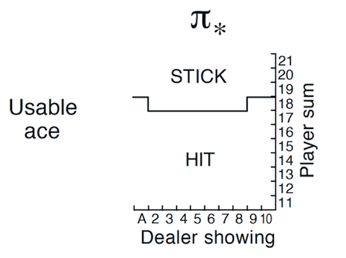
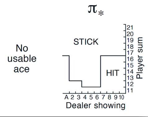
下图是有Usable Ace情况下的理论最优策略。
理论最佳策略(有Ace)
Monte 
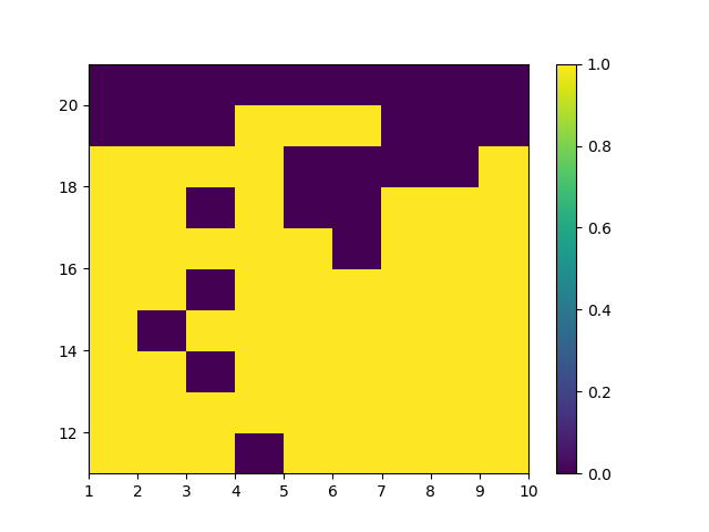
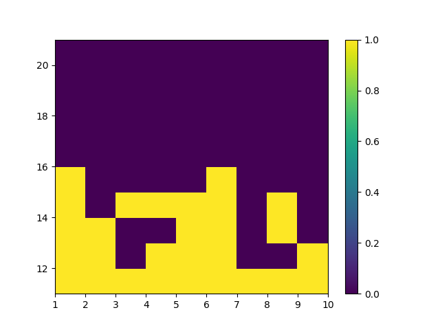
Carlo方法策略提示的收敛是比较慢的,下图是运行10,000,000次episode后有Usable Ace时的策略 \(\pi_{*}^{\prime}\)。对比理论最优策略,MC ES在不少的状态下还未收敛到理论最优解。
MC ES 10M的最佳策略(有Ace)
同样的,下两张图是无Usable Ace情况下的理论最优策略和试验结果的对比。
理论最佳策略(无Ace)
MC ES 10M的最佳策略(无Ace)
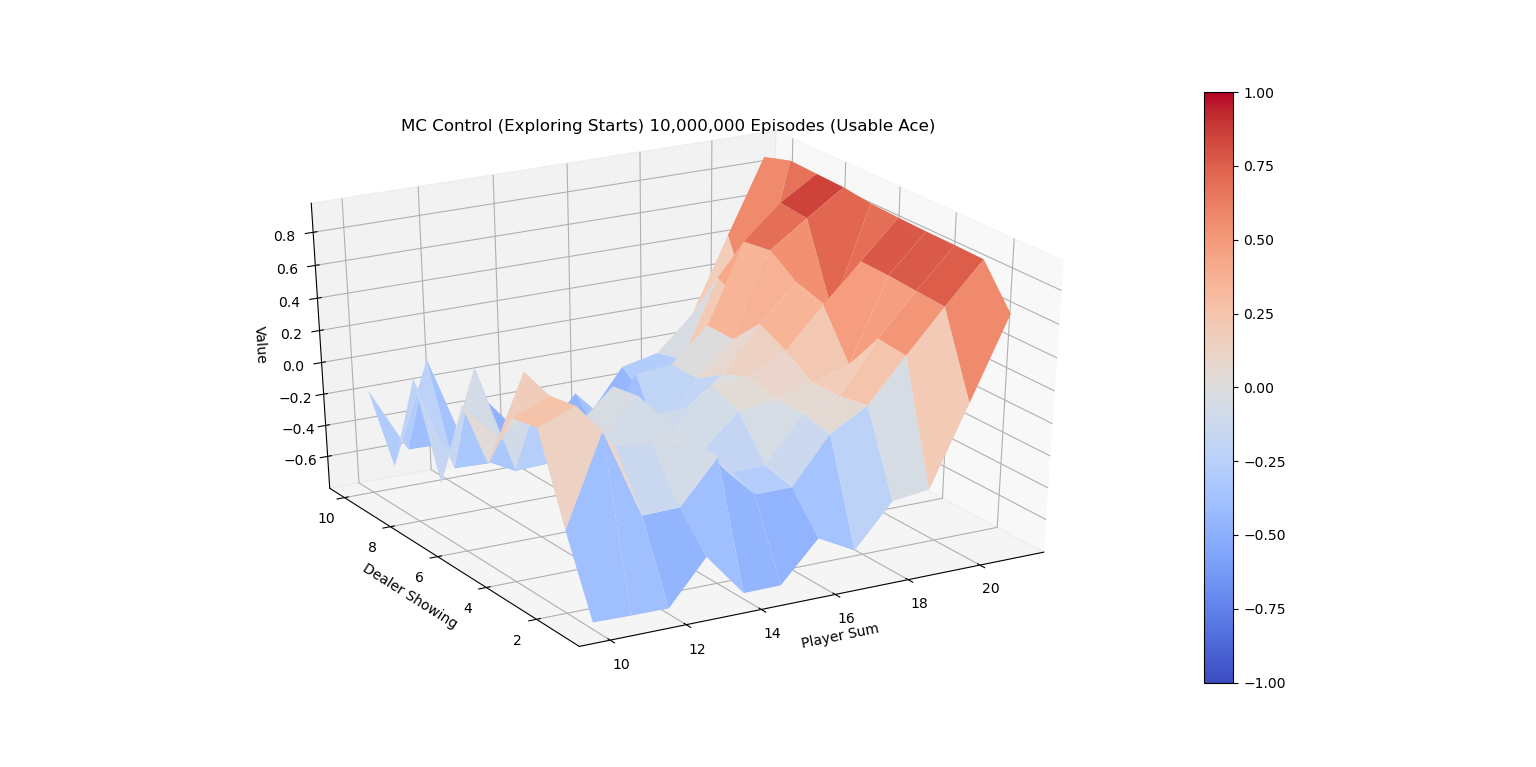
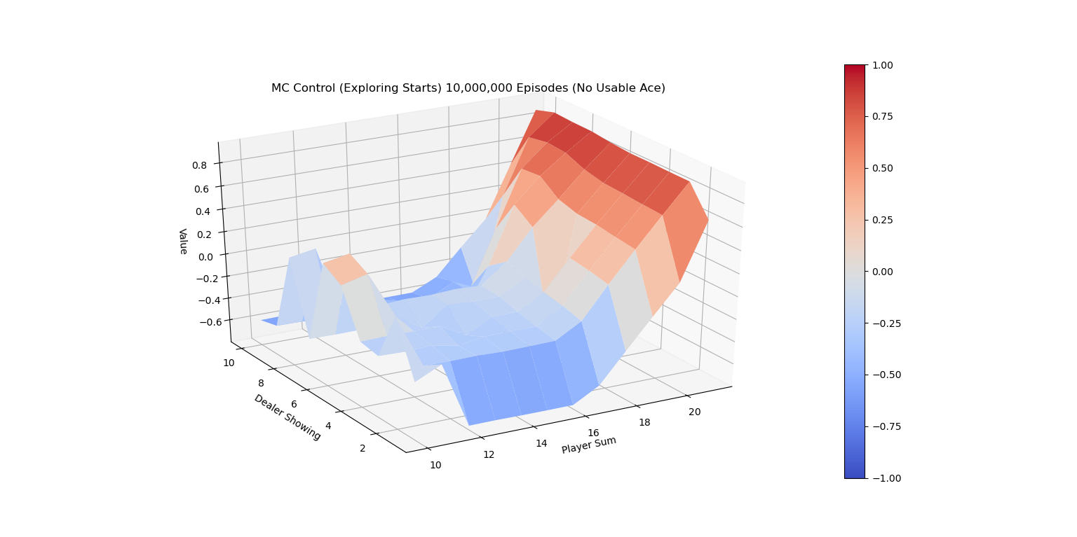
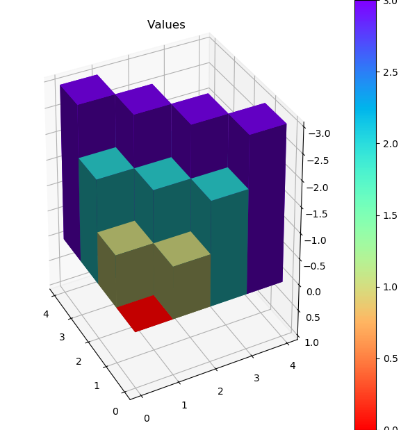
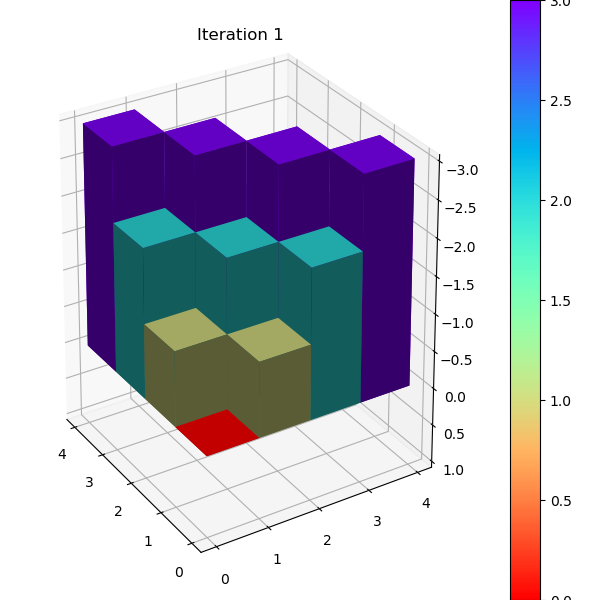
下面的两张图画出了运行代码10,000,000次episode后 \(\pi{*}\)的V值图。
MC ES 10M的最佳V值(有Ace)
MC ES 10M的最佳V值(无Ace)

Exploring Starts 蒙特卡洛控制改进

为了避免Monte Carlo ES Control在初始时必须访问到任意状态的限制,教材中介绍了一种改进算法,On-policy first-visit MC control for \(\epsilon \text{-soft policies}\) ,它同样基于Monte Carlo 预估Q值,但用 \(\epsilon \text{-soft}\) 策略来代替最有可能的action策略作为下一次迭代策略,\(\epsilon \text{-soft}\) 本质上来说就是对于任意动作都保留 \(\epsilon\) 小概率的访问可能,权衡了exploration和exploitation,由于每个动作都可能被无限次访问到,Explorting Starts中的强制随机初始状态就可以去除了。Monte Carlo ES Control 和 On-policy first-visit MC control for \(\epsilon \text{-soft policies}\) 都属于on-policy算法,其区别于off-policy的本质在于预估 \(q_{\pi}(s,a)\)时是否从同策略\(\pi\)生成的数据来计算。一个比较subtle的例子是著名的Q-Learning,因为根据这个定义,Q-Learning属于off-policy。

\[ \begin{align*} &\textbf{On-policy first-visit MC control (for }\epsilon \textbf{-soft policies), estimating } \pi \approx \pi_{*} \\ & \text{Algorithm parameter: small } \epsilon > 0 \\ & \text{Initialize:} \\ & \quad \pi \leftarrow \text{ an arbitrary } \epsilon \text{-soft policy} \\ & \quad Q(s, a) \in \mathbb R \text{, arbitrarily, for all }s \in \mathcal{S}, a \in \mathcal A(s) \\ & \quad Returns(s, a) \leftarrow \text{ an empty list, for all }s \in \mathcal{S}, a \in \mathcal A(s)\\ & \\ & \text{Repeat forever (for episode):}\\ & \quad \text{Generate an episode following } \pi : S_0, A_0, R_1, S_1, A_1, R_2, ..., S_{T-1}, A_{T-1}, R_T\\ & \quad G \leftarrow 0\\ & \quad \text{Loop for each step of episode, } t = T-1, T-2, ..., 0:\\ & \quad \quad \quad G \leftarrow \gamma G + R_{t+1}\\ & \quad \quad \quad \text{Unless the pair } S_t, A_t \text{ appears in } S_0, A_0, S_1, A_1, ..., S_{t-1}, A_{t-1}\\ & \quad \quad \quad \quad \text{Append } G \text { to }Returns(S_t, A_t) \\ & \quad \quad \quad \quad Q(S_t, A_t) \leftarrow \operatorname{average}(Returns(S_t, A_t))\\ & \quad \quad \quad \quad A^{*} \leftarrow \operatorname{argmax}_a Q(S_t, a)\\ & \quad \quad \quad \quad \text{For all } a \in \mathcal A(S_t):\\ & \quad \quad \quad \quad \quad \pi(a|S_t) \leftarrow \begin{cases} 1 - \epsilon + \epsilon / |\mathcal A(S_t)| & \text{ if } a = A^{*}\\ \epsilon / |\mathcal A(S_t)| & \text{ if } a \neq A^{*}\\ \end{cases} \\ \end{align*} \]

伪代码对应的 Python 实现如下。

{linenos
1
2
3
4
5
6
7
8
9
10
11
12
13
14
15
16
17
18
19
20
21
22
23
24
25
26
27
28
def mc_control_epsilon_greedy(env: BlackjackEnv, num_episodes, discount_factor=1.0, epsilon=0.1) \
-> Tuple[ActionValue, Policy]:
returns_sum = defaultdict(float)
returns_count = defaultdict(float)

states = list(product(range(10, 22), range(1, 11), (True, False)))
policy = {s: np.ones(env.action_space.n) * 1.0 / env.action_space.n for s in states}
Q = defaultdict(lambda: np.zeros(env.action_space.n))

def update_epsilon_greedy_policy(policy: Policy, Q: ActionValue, s: State):
policy[s] = np.ones(env.action_space.n, dtype=float) * epsilon / env.action_space.n
best_action = np.argmax(Q[s])
policy[s][best_action] += (1.0 - epsilon)

for episode_i in range(1, num_episodes + 1):
episode_history = gen_stochastic_episode(policy, env)

G = 0
for t in range(len(episode_history) - 1, -1, -1):
s, a, r = episode_history[t]
G = discount_factor * G + r
if not any(s_a_r[0] == s and s_a_r[1] == a for s_a_r in episode_history[0: t]):
returns_sum[s, a] += G
returns_count[s, a] += 1.0
Q[s][a] = returns_sum[s, a] / returns_count[s, a]
update_epsilon_greedy_policy(policy, Q, s)

return Q, policy

从这期开始我们进入Sutton强化学习第二版,第五章蒙特卡洛方法。蒙特卡洛方法是一种在工程各领域都存在的基本方法,在强化领域中,其特点是无需知道环境的dynamics,只需不断模拟记录并分析数据即可逼近理论真实值。蒙特卡洛方法本篇将会用21点游戏作为示例来具体讲解其原理和代码实现。

21点游戏问题

21点游戏是一个经典的赌博游戏。大致规则是玩家和庄家各发两张牌,一张明牌,一张暗牌。玩家和庄家可以决定加牌或停止加牌,新加的牌均为暗牌,最后比较两个玩家的牌面和,更接近21点的获胜。游戏的变化因素是牌Ace,既可以作为11也可以作为1来计算,算作11的时候称作usable。

Sutton教材中的21点游戏规则简化了几个方面用于控制问题状态数:

  • 已发的牌的无状态性:和一副牌的21点游戏不同的是,游戏环境简化为牌是可以无穷尽被补充的,一副牌的某一张被派发后,同样的牌会被补充进来,或者可以认为每次发放的牌都是从一副新牌中抽出的。统计学中的术语称为重复采样(sample with replacement)。这种规则下极端情况下,玩家可以拥有 5个A或者5个2。另外,这会导致玩家无法通过开局看到的3张牌的信息推断后续发牌的概率,如此就大规模减小了游戏状态数。
  • 庄家和玩家独立游戏,无需按轮次要牌。开局给定4张牌后,玩家先行动,加牌直至超21点或者停止要牌,如果超21点,玩家输,否则,等待庄家行动,庄家加牌直至超21点或者停止要牌,如果超21点,庄家输,否则比较两者的总点数。这种方式可以认为当玩家和庄家看到初始的三张牌后独立做一系列决策,最后比较结果,避免了交互模式下因为能观察到每一轮后对方牌数变化产生额外的信息而导致的游戏状态数爆炸。

有以上两个规则的简化,21点游戏问题的总状态数有下面三个维度

  • 自己手中的点数和(12到21)

  • 庄家明牌的点数(A到10)

  • 庄家明牌是否有 A(True, False)。

状态总计总数为三个维度的乘积 10 * 10 * 2 = 200。

关于游戏状态有几个比较subtle的假设或者要素。首先,玩家初始时能看到三张牌,这三张牌确定了状态的三个维度的值,当然也就确定了Agent的初始状态,随后按照独立游戏的规则进行,玩家根据初始状态依照某种策略决策要牌还是结束要牌,新拿的牌更新了游戏状态,玩家转移到新状态下继续做决策。举个例子,假设初始时玩家明牌为8,暗牌为6,庄家明牌为7,则游戏状态为Tuple (14, 7, False)。若玩家的策略为教材中的固定规则策略:没到20或者21继续要牌。下一步玩家拿到牌3,则此时新状态为 (17, 7, False),按照策略继续要牌。

第二个方面是游戏的状态完全等价于玩家观察到的信息。比如尽管初始时有4张牌,真正的状态是这四张牌的值,但是出于简化目的,不考虑partially observable 的情况,即不将暗牌纳入游戏状态中。另外,庄家做决策的时候也无法得知玩家的手中的总牌数。

第三个方面是关于玩家点数。考虑玩家初始时的两张牌为2,3,总点数是5,那么为何不将5加入到游戏状态中呢?原则上是可以将初始总和为2到11都加入到游戏状态,但是意义不大,原因在于我们已经假设了已发牌的无状态性,拿到的这两张牌并不会改变后续补充的牌的出现概率。当玩家初始总和为2到11时一定会追加牌,因为无论第三张牌是什么,都不会超过21点,只会增加获胜概率。若后续第三张牌为8,总和变成13,就进入了有效的游戏状态,因为此时如果继续要牌,获得10,则游戏输掉。因此,我们关心的游戏状态并不完全等价于所有可能的游戏状态。

21点游戏 OpenAI Gym环境

OpenAI Gym 已经实现了Sutton版本的21点游戏环境,并按上述规则来进行。在安装完OpenAI Gym包之后 import BlackjackEnv即可使用。

1
from gym.envs.toy_text import BlackjackEnv

根据这个游戏环境,我们先来定义一些类型,可以令代码更具可读性和抽象化。State 上文说过是由三个分量组成的Tuple。Action 为bool类型 表示是否继续要牌。Reward 为+1或者-1,玩家叫牌过程中为0。StateValue 为书中的 \(V_{\pi}\),实现上是一个Dict。DeterministicPolicy 为一个函数,输入是某一状态,输出是唯一的决策动作。

{linenos
1
2
3
4
5
State = Tuple[int, int, bool]
Action = bool
Reward = float
StateValue = Dict[State, float]
DeterministicPolicy = Callable[[State], Action]

以下代码是 BlackjackEnv 核心代码,step 方法的输入为玩家的决策动作(叫牌还是结束),并输出State, Reward, is_done。简单解释一下代码逻辑,当玩家继续加牌时,需要判断是否超21点,如果没有超过的话,返回下一状态,同时reward 为0,等待下一step方法。若玩家停止叫牌,则按照庄家策略:小于17时叫牌。游戏终局时产生+1表示玩家获胜,-1表示庄家获胜。

{linenos
1
2
3
4
5
6
7
8
9
10
11
12
13
14
15
16
17
18
19
20
21
22
23
class BlackjackEnv(gym.Env):

def step(self, action):
assert self.action_space.contains(action)
if action: # hit: add a card to players hand and return
self.player.append(draw_card(self.np_random))
if is_bust(self.player):
done = True
reward = -1.
else:
done = False
reward = 0.
else: # stick: play out the dealers hand, and score
done = True
while sum_hand(self.dealer) < 17:
self.dealer.append(draw_card(self.np_random))
reward = cmp(score(self.player), score(self.dealer))
if self.natural and is_natural(self.player) and reward == 1.:
reward = 1.5
return self._get_obs(), reward, done, {}

def _get_obs(self):
return (sum_hand(self.player), self.dealer[0], usable_ace(self.player))

下面示例如何调用step方法生成一个episode的数据集。数据集的类型为 List[Tuple[State, Action, Reward]]。

{linenos
1
2
3
4
5
6
7
8
9
10
def gen_episode_data(policy: DeterministicPolicy, env: BlackjackEnv) -> List[Tuple[State, Action, Reward]]:
episode_history = []
state = env.reset()
done = False
while not done:
action = policy(state)
next_state, reward, done, _ = env.step(action)
episode_history.append((state, action, reward))
state = next_state
return episode_history

策略的蒙特卡洛值预测

Monte Carlo Prediction解决如下问题:当给定Agent 策略\(\pi\)时,反复试验来预估策略的 \(V_{\pi}\) 值。具体来说,产生一系列的episode数据之后,对于出现了的所有状态分别计算其Return,再通过 average 某一状态 s 的Return来估计 \(V_{\pi}(s)\),理论上,依据大数定理(Law of large numbers),在可以无限模拟的情况下,Monte Carlo prediction 一定会收敛到真实的 \(V_{\pi}\)。算法实现上有两个略微不同的版本,一个版本称为 First-visit,另一个版本称为 Every-visit,区别在于如何计算出现的状态 s 的 Return值。

对于 First-visit 来说,当状态 s 第一次出现时计算一次 Returns,若继续出现状态 s 不再重复计算。对于Every-visit来说,每次出现 s 计算一次 Returns(s)。举个例子,某episode 数据如下: \[ S_1, R_1, S_2, R_2, S_1, R_3, S_3, R_4 \] First-visit 对于状态S1的Returns计算为

\[ Returns(S_1) = R_1 + R_2 + R_3 + R_4 \]

Every-visit 对于状态S1的Returns计算了两次,因为S1出现了两次。 \[ \begin{align*} Returns(S_1) = \frac{Return_1(S_1) + Return_2(S_1)}2 \\ = \frac{(R_1 + R_2 + R_3 + R_4) + (R_3 + R_4)} 2 \end{align*} \]

下面用Monte Carlo来模拟解得书中示例玩家固定策略的V值,策略具体为:加牌直到手中点数>=20,代码为

{linenos
1
2
3
4
5
6
def fixed_policy(observation):
"""
sticks if the player score is >= 20 and hits otherwise.
"""
score, dealer_score, usable_ace = observation
return 0 if score >= 20 else 1

First-visit MC Predicition

伪代码如下,注意考虑到实现上的高效性,在遍历episode序列数据时是从后向前扫的,这样可以边扫边更新G。

\[ \begin{align*} &\textbf{First-visit MC prediction, for estimating } V \approx v_{\pi} \\ & \text{Input: a policy } \pi \text{ to be evaluated} \\ & \text{Initialize} \\ & \quad V(s) \in \mathbb R \text{, arbitrarily, for all }s \in \mathcal{S} \\ & \quad Returns(s) \leftarrow \text{ an empty list, arbitrarily, for all }s \in \mathcal{S} \\ & \\ & \text{Loop forever (for episode):}\\ & \quad \text{Generate an episode following } \pi: S_0, A_0, R_1, S_1, A_1, R_2, ..., S_{T-1}, A_{T-1}, R_T\\ & \quad G \leftarrow 0\\ & \quad \text{Loop for each step of episode, } t = T-1, T-2, ..., 0:\\ & \quad \quad \quad G \leftarrow \gamma G + R_{t+1}\\ & \quad \quad \quad \text{Unless } S_t \text{ appears in } S_0, S_1, ..., S_{t-1}\\ & \quad \quad \quad \quad \text{Append } G \text { to }Returns(S_t) \\ & \quad \quad \quad \quad V(S_t) \leftarrow \operatorname{average}(Returns(S_t))\\ \end{align*} \]

对应的 python 实现

{linenos
1
2
3
4
5
6
7
8
9
10
11
12
13
14
15
16
17
18
19
def mc_prediction_first_visit(policy: DeterministicPolicy, env: BlackjackEnv,
num_episodes, discount_factor=1.0) -> StateValue:
returns_sum = defaultdict(float)
returns_count = defaultdict(float)

for episode_i in range(1, num_episodes + 1):
episode_history = gen_episode_data(policy, env)

G = 0
for t in range(len(episode_history) - 1, -1, -1):
s, a, r = episode_history[t]
G = discount_factor * G + r
if not any(s_a_r[0] == s for s_a_r in episode_history[0: t]):
returns_sum[s] += G
returns_count[s] += 1.0

V = defaultdict(float)
V.update({s: returns_sum[s] / returns_count[s] for s in returns_sum.keys()})
return V

Every-visit MC Prediciton

Every-visit 代码实现相对更简单一些,t 从后往前遍历时更新对应s的状态变量。如下所示

{linenos
1
2
3
4
5
6
7
8
9
10
11
12
13
14
15
16
17
18
def mc_prediction_every_visit(policy: DeterministicPolicy, env: BlackjackEnv,
num_episodes, discount_factor=1.0) -> StateValue:
returns_sum = defaultdict(float)
returns_count = defaultdict(float)

for episode_i in range(1, num_episodes + 1):
episode_history = gen_episode_data(policy, env)

G = 0
for t in range(len(episode_history) - 1, -1, -1):
s, a, r = episode_history[t]
G = discount_factor * G + r
returns_sum[s] += G
returns_count[s] += 1.0

V = defaultdict(float)
V.update({s: returns_sum[s] / returns_count[s] for s in returns_sum.keys()})
return V

策略 V值 3D 可视化

运行first-visit 算法,模拟10000次episode,fixed_policy的V值的3D图为下面两张图,分别是不含usable Ace和包含usable Ace。总的说来,一旦玩家能到达20点或21点获胜概率极大,到达13-17获胜概率较小,在11-13时有一定获胜概率,比较符合经验直觉。

first-visit MC 10000次没有usable A的V值
first-visit MC 10000次含有usable A的V值

同样运行every-visit 算法,模拟10000次的V值图。对比两种方法结果比较接近。

every-visit MC 10000次没有usable A的V值
every-visit MC 10000次含有usable A的V值

本篇是TSP问题从DP算法到深度学习系列第二篇。

AIZU TSP 自底向上迭代DP解

上一篇中,我们用Python 3和Java 8完成了自顶向下递归版本的DP解。我们继续改进代码,将它转换成标准DP方式:自底向上的迭代DP版本。下图是3个点TSP问题的递归调用图。

将这个图反过来检查状态的依赖关系,可以很容易发现规律:首先计算状态位含有一个1的点,接着是两个1的节点,最后是状态位三个1的点。简而言之,在计算状态位为n+1个1的节点时需要用到n个1的节点的计算结果,如果能依照这样的 topological 顺序来的话,就可以去除递归,写成迭代(循环)版本的DP。

迭代算法的Java 伪代码如下

1
2
3
4
5
6
7
8
9
10
11
12
13
14
15
16
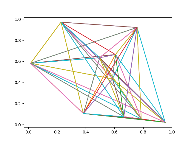
for (int bitset_num = N; bitset_num >=0; bitset_num++) {
while(hasNextCombination(bitset_num)) {
int state = nextCombination(bitset_num);
// compute dp[state][v], v-th bit is set in state
for (int v = 0; v < n; v++) {
for (int u = 0; u < n; u++) {
// for each u not reached by this state
if (!include(state, u)) {
dp[state][v] = min(dp[state][v],
dp[new_state_include_u][u] + dist[v][u]);
}
}
}
}
}

举例来说,dp[00010][1] 是从顶点0出发,刚经过顶点1的最小距离 \(0 \rightarrow 1 \rightarrow ? \rightarrow ? \rightarrow ? \rightarrow 0\)

为了找到最小距离值,就必须遍历所有可能的下一个可能的顶点u (第一个问号位置)。 \[ (0 \rightarrow 1) + \begin{align*} \min \left\lbrace \begin{array}{r@{}l} 2 \rightarrow ? \rightarrow ? \rightarrow 0 + dist(1,2) \qquad\text{ new_state=[00110][2] } \qquad\\\\ 3 \rightarrow ? \rightarrow ? \rightarrow 0 + dist(1,3) \qquad\text{ new_state=[01010][3] } \qquad\\\\ 4 \rightarrow ? \rightarrow ? \rightarrow 0 + dist(1,4) \qquad\text{ new_state=[10010][4] } \qquad \end{array} \right. \end{align*} \]

迭代DP AC代码

以下是AC 的Java 算法核心代码。完整代码在 github/MyEncyclopedia 的tsp/alg_aizu/Main_loop.java

{linenos
1
2
3
4
5
6
7
8
9
10
11
12
13
14
15
16
17
18
19
20
public long solve() {
int N = g.V_NUM;
long[][] dp = new long[1 << N][N];
// init dp[][] with MAX
for (int i = 0; i < dp.length; i++) {
Arrays.fill(dp[i], Integer.MAX_VALUE);
}
dp[(1 << N) - 1][0] = 0;

for (int state = (1 << N) - 2; state >= 0; state--) {
for (int v = 0; v < N; v++) {
for (int u = 0; u < N; u++) {
if (((state >> u) & 1) == 0) {
dp[state][v] = Math.min(dp[state][v], dp[state | 1 << u][u] + g.edges[v][u]);
}
}
}
}
return dp[0][0] == Integer.MAX_VALUE ? -1 : dp[0][0];
}

很显然,时间算法复杂度对应了三重 for 循环,为 O(\(2^n * n * n\)) = O(\(2^n*n^2\) )。

类似的,Python 3 AC 代码如下。完整代码在 github/MyEncyclopedia 的tsp/alg_aizu/TSP_loop.py

{linenos
1
2
3
4
5
6
7
8
9
10
11
12
13
14
15
16
17
18
19
20
21
22
23
24
25
26
27
class TSPSolver:
g: Graph

def __init__(self, g: Graph):
self.g = g

def solve(self) -> int:
"""
:param v:
:param state:
:return: -1 means INF
"""
N = self.g.v_num
dp = [[INT_INF for c in range(N)] for r in range(1 << N)]

dp[(1 << N) - 1][0] = 0

for state in range((1 << N) - 2, -1, -1):
for v in range(N):
for u in range(N):
if ((state >> u) & 1) == 0:
if dp[state | 1 << u][u] != INT_INF and self.g.edges[v][u] != INT_INF:
if dp[state][v] == INT_INF:
dp[state][v] = dp[state | 1 << u][u] + self.g.edges[v][u]
else:
dp[state][v] = min(dp[state][v], dp[state | 1 << u][u] + self.g.edges[v][u])
return dp[0][0]

一个欧式空间TSP数据集

至此,TSP的DP解法全部讲解完毕。接下去,我们引入一个二维欧式空间的TSP数据集 PTR_NET on Google Drive ,这个数据集是 Pointer Networks 的作者 Oriol Vinyals 用于模型的训练测试而引入的。

数据集的每一行格式如下:

1
x1, y1, x2, y2, ... output 1 v1 v2 v3 ... 1

一行开始为n个点的x, y坐标,接着是 output,再接着是1,表示从顶点1出发,经v1,v2,...,返回1,注意顶点编号从1开始。

十个顶点数据集的一些数据示例如下:

1
2
3
4
0.607122 0.664447 0.953593 0.021519 0.757626 0.921024 0.586376 0.433565 0.786837 0.052959 0.016088 0.581436 0.496714 0.633571 0.227777 0.971433 0.665490 0.074331 0.383556 0.104392 output 1 3 8 6 10 9 5 2 4 7 1 
0.930534 0.747036 0.277412 0.938252 0.794592 0.794285 0.961946 0.261223 0.070796 0.384302 0.097035 0.796306 0.452332 0.412415 0.341413 0.566108 0.247172 0.890329 0.429978 0.232970 output 1 3 2 9 6 5 8 7 10 4 1
0.686712 0.087942 0.443054 0.277818 0.494769 0.985289 0.559706 0.861138 0.532884 0.351913 0.712561 0.199273 0.554681 0.657214 0.909986 0.277141 0.931064 0.639287 0.398927 0.406909 output 1 5 2 10 7 4 3 9 8 6 1

画出第一个例子的全部顶点和边。

{linenos
1
2
3
4
5
6
7
8
9
10
11
12
13
14
15
16
17
18
import matplotlib.pyplot as plt
points='0.607122 0.664447 0.953593 0.021519 0.757626 0.921024 0.586376 0.433565 0.786837 0.052959 0.016088 0.581436 0.496714 0.633571 0.227777 0.971433 0.665490 0.074331 0.383556 0.104392'
float_list = list(map(lambda x: float(x), points.split(' ')))

x,y = [],[]
for idx, p in enumerate(float_list):
if idx % 2 == 0:
x.append(p)
else:
y.append(p)

for i in range(0, len(x)):
for j in range(0, len(x)):
if i == j:
continue
plt.plot((x[i],x[j]),(y[i],y[j]))

plt.show()
全连接的图

这个例子的最短TSP旅程为 \[ 1 \rightarrow 3 \rightarrow 8 \rightarrow 6 \rightarrow 10 \rightarrow 9 \rightarrow 5 \rightarrow 2 \rightarrow 4 \rightarrow 7 \rightarrow 1 \]

{linenos
1
2
3
4
5
6
7
8
tour_str = '1 3 8 6 10 9 5 2 4 7 1'
tour = list(map(lambda x: int(x), tour_str.split(' ')))

for i in range(0, len(tour)-1):
p1 = tour[i] - 1
p2 = tour[i + 1] - 1
plt.plot((x[p1],x[p2]),(y[p1],y[p2]))
plt.show()
最短路径

PTR_NET TSP 的Python代码

初始化Init Graph Edges

在之前的自顶向下的递归版本中,需要做一些改动。首先,是图的初始化,我们依然延续之前的邻接矩阵来表示,由于这次的图是无向图,对于任意两个顶点,需要初始化双向的边。

{linenos
1
2
3
4
5
6
7
8
g: Graph = Graph(N)
for v in range(N):
for u in range(N):
diff_x = coordinates[v][0] - coordinates[u][0]
diff_y = coordinates[v][1] - coordinates[u][1]
dist: float = math.sqrt(diff_x * diff_x + diff_y * diff_y)
g.setDist(u, v, dist)
g.setDist(v, u, dist)

辅助变量记录父节点

另一大改动是需要在遍历过程中保存的顶点关联信息,以便在最终找到最短路径值时可以回溯对应的完整路径。在下面代码中,使用parent[bitstate][v] 来保存此状态下最小路径对应的顶点u。

{linenos
1
2
3
4
5
6
7
8
9
10
11
ret: float = FLOAT_INF
u_min: int = -1
for u in range(self.g.v_num):
if (state & (1 << u)) == 0:
s: float = self._recurse(u, state | 1 << u)
if s + edges[v][u] < ret:
ret = s + edges[v][u]
u_min = u
dp[state][v] = ret
self.parent[state][v] = u_min

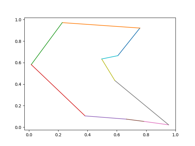
当最终最短行程确定后,根据parent的信息可以按图索骥找到完整的行程顶点信息。

{linenos
1
2
3
4
5
6
7
8
9
def _form_tour(self):
self.tour = [0]
bit = 0
v = 0
for _ in range(self.g.v_num - 1):
v = self.parent[bit][v]
self.tour.append(v)
bit = bit | (1 << v)
self.tour.append(0)

需要注意的是,有可能存在多个最短行程,它们的距离值是一致的。这种情况下,代码输出的最短路径可能和数据集output后行程路径不一致,但是的两者的总距离是一致的。下面的代码验证了这一点。

{linenos
1
2
3
4
5
6
7
8
9
10
11
12
13
14
15
16
17
18
tsp: TSPSolver = TSPSolver(g)
tsp.solve()

output_dist: float = 0.0
output_tour = list(map(lambda x: int(x) - 1, output.split(' ')))
for v in range(1, len(output_tour)):
pre_v = output_tour[v-1]
curr_v = output_tour[v]
diff_x = coordinates[pre_v][0] - coordinates[curr_v][0]
diff_y = coordinates[pre_v][1] - coordinates[curr_v][1]
dist: float = math.sqrt(diff_x * diff_x + diff_y * diff_y)
output_dist += dist

passed = abs(tsp.dist - output_dist) < 10e-5
if passed:
print(f'passed dist={tsp.tour}')
else:
print(f'Min Tour Distance = {output_dist}, Computed Tour Distance = {tsp.dist}, Expected Tour = {output_tour}, Result = {tsp.tour}')

本文所有代码在 github/MyEncyclopedia tsp/alg_plane 中。

上一期 通过代码学Sutton强化学习1:Grid World OpenAI环境和策略评价算法,我们引入了 Grid World 问题,实现了对应的OpenAI Gym 环境,也分析了其最佳策略和对应的V值。这一期中,继续通过这个例子详细讲解策略提升(Policy Improvment)、策略迭代(Policy Iteration)、值迭代(Value Iteration)和异步迭代方法。

回顾 Grid World 问题

Grid World 问题
在Grid World 中,Agent初始可以出现在编号1-14的网格中,Agent 每往四周走一步得到 -1 reward,因此需要尽快走到两个出口。当然最佳策略是以最小步数往出口逃离,如下所示。
Grid World 最佳策略

最佳策略对应的状态V值和3D heatmap如下

1
2
3
4
[[ 0. -1. -2. -3.]
[-1. -2. -3. -2.]
[-2. -3. -2. -1.]
[-3. -2. -1. 0.]]

Grid World V值 3D heatmap

策略迭代

上一篇中,我们知道如何evaluate 给定policy \(\pi\)\(v_{\pi}\)值,那么是否可能在此基础上改进生成更好的策略 \(\pi^{\prime}\)。如果可以,能否最终找到最佳策略\({\pi}_{*}\)?答案是肯定的,因为存在策略提升定理(Policy Improvement Theorem)。

策略提升定理

在 4.2 节 Policy Improvement Theorem 可以证明,利用 \(v_{\pi}\) 信息对于每个状态采取最 greedy 的 action (又称exploitation)能够保证生成的新 \({\pi}^{\prime}\) 是不差于旧的policy \({\pi}\),即

\[ q_{\pi}(s, {\pi}^{\prime}(s)) \gt v_{\pi}(s) \]

\[ v_{\pi^{\prime}}(s) \gt v_{\pi}(s) \]

因此,可以通过在当前policy求得v值,再选取最greedy action的方式形成如下迭代,就能够不断逼近最佳策略。

\[ \pi_{0} \stackrel{\mathrm{E}}{\longrightarrow} v_{\pi_{0}} \stackrel{\mathrm{I}}{\longrightarrow} \pi_{1} \stackrel{\mathrm{E}}{\longrightarrow} v_{\pi_{1}} \stackrel{\mathrm{I}}{\longrightarrow} \pi_{2} \stackrel{\mathrm{E}}{\longrightarrow} \cdots \stackrel{\mathrm{I}}{\longrightarrow} \pi_{*} \stackrel{\mathrm{E}}{\longrightarrow} v_{*} \]

策略迭代算法

以下为书中4.3的policy iteration伪代码。其中policy evaluation的算法在上一篇中已经实现。Policy improvement 的精髓在于一次遍历所有状态后,通过policy 的最大Q值找到该状态的最佳action,并更新成最新policy,循环直至没有 action 变更。

\[ \begin{align*} &\textbf{Policy Iteration (using iterative policy evaluation) for estimating } \pi\approx {\pi}_{*} \\ &1. \quad \text{Initialization} \\ & \quad \quad V(s) \in \mathbb R\text{ and } \pi(s) \in \mathcal A(s) \text{ arbitrarily for all }s \in \mathcal{S} \\ & \\ &2. \quad \text{Policy Evaluation} \\ & \quad \quad \text{Loop:}\\ & \quad \quad \Delta \leftarrow 0\\ & \quad \quad \text{Loop for each } s \in \mathcal{S}:\\ & \quad \quad \quad \quad v \leftarrow V(s) \\ & \quad \quad \quad \quad V(s) \leftarrow \sum_{s^{\prime}, r} p\left(s^{\prime}, r \mid s, a\right)\left[r+\gamma V\left(s^{\prime}\right)\right] \\ & \quad \quad \quad \quad \Delta \leftarrow \max(\Delta, |v-V(s)|) \\ & \quad \quad \text{until } \Delta < \theta \text{ (a small positive number determining the accuracy of estimation)}\\ & \\ &3. \quad \text{Policy Improvement} \\ & \quad \quad policy\text{-}stable\leftarrow true \\ & \quad \quad \text{Loop for each } s \in \mathcal{S}:\\ & \quad \quad \quad \quad old\text{-}action\leftarrow \pi(s) \\ & \quad \quad \quad \quad \pi(s) \leftarrow \operatorname{argmax}_{a} \sum_{s^{\prime}, r} p\left(s^{\prime}, r \mid s, a\right)\left[r+\gamma V\left(s^{\prime}\right)\right] \\ & \quad \quad \quad \quad \text{If } old\text{-}action \neq \pi\text{,then }policy\text{-}stable\leftarrow false \\ & \quad \quad \text{If } policy\text{-}stable \text{, then stop and return }V \approx v_{*} \text{ and } \pi\approx {\pi}_{*}\text{; else go to 2} \end{align*} \]

注意到状态Q值 \(q_{\pi}(s, a)\) 会被多处调用,将其封装为单独的函数。

\[ \begin{aligned} q_{\pi}(s, a) &=\sum_{s^{\prime}, r} p\left(s^{\prime}, r \mid s, a\right)\left[r+\gamma v_{\pi}\left(s^{\prime}\right)\right] \end{aligned} \]

Q值函数实现如下:

{linenos
1
2
3
4
5
6
def action_value(env: GridWorldEnv, state: State, V: StateValue, gamma=1.0) -> ActionValue:
q = np.zeros(env.nA)
for a in range(env.nA):
for prob, next_state, reward, done in env.P[state][a]:
q[a] += prob * (reward + gamma * V[next_state])
return q

有了 action_value 和上期的 policy_evaluate,policy iteration 实现完全对应上面的伪代码。

{linenos
1
2
3
4
5
6
7
8
9
10
11
12
13
14
15
16
17
18
19
20
21
22
23
def policy_improvement(env: GridWorldEnv, policy: Policy, V: StateValue, gamma=1.0) -> bool:
policy_stable = True

for s in range(env.nS):
old_action = np.argmax(policy[s])
Q_s = action_value(env, s, V)
best_action = np.argmax(Q_s)
policy[s] = np.eye(env.nA)[best_action]

if old_action != best_action:
policy_stable = False
return policy_stable


def policy_iteration(env: GridWorldEnv, policy: Policy, gamma=1.0) -> Tuple[Policy, StateValue]:
iter = 0
while True:
V = policy_evaluate(policy, env, gamma)
policy_stable = policy_improvement(env, policy, V)
iter += 1

if policy_stable:
return policy, V

Grid World 例子通过两轮迭代就可以收敛,以下是初始时随机策略的V值和第一次迭代后的V值。
初始随机策略 V 值
第一次迭代后的 V 值

值迭代

值迭代( Value Iteration)的本质是,将policy iteration中的policy evaluation过程从不断循环到收敛直至小于theta,改成只执行一遍,并直接用最佳Q值更新到状态V值,如此可以不用显示地算出\({\pi}\) 而直接在V值上迭代。具体迭代公式如下:

\[ \begin{aligned} v_{k+1}(s) & \doteq \max _{a} \mathbb{E}\left[R_{t+1}+\gamma v_{k}\left(S_{t+1}\right) \mid S_{t}=s, A_{t}=a\right] \\ &=\max_{a} q_{\pi_k}(s, a) \\ &=\max _{a} \sum_{s^{\prime}, r} p\left(s^{\prime}, r \mid s, a\right)\left[r+\gamma v_{k}\left(s^{\prime}\right)\right] \end{aligned} \]

完整的伪代码为:

\[ \begin{align*} &\textbf{Value Iteration, for estimating } \pi\approx \pi_{*} \\ & \text{Algorithm parameter: a small threshold } \theta > 0 \text{ determining accuracy of estimation} \\ & \text{Initialize } V(s), \text{for all } s \in \mathcal{S}^{+} \text{, arbitrarily except that } V (terminal) = 0\\ & \\ &1: \text{Loop:}\\ &2: \quad \quad \Delta \leftarrow 0\\ &3: \quad \quad \text{Loop for each } s \in \mathcal{S}:\\ &4: \quad \quad \quad \quad v \leftarrow V(s) \\ &5: \quad \quad \quad \quad V(s) \leftarrow \operatorname{max}_{a} \sum_{s^{\prime}, r} p\left(s^{\prime}, r \mid s, a\right)\left[r+\gamma V\left(s^{\prime}\right)\right] \\ &6: \quad \quad \quad \quad \Delta \leftarrow \max(\Delta, |v-V(s)|) \\ &7: \text{until } \Delta < \theta \\ & \\ & \text{Output a deterministic policy, }\pi\approx \pi_{*} \text{, such that} \\ & \quad \quad \pi(s) \leftarrow \operatorname{argmax}_{a} \sum_{s^{\prime}, r} p\left(s^{\prime}, r \mid s, a\right)\left[r+\gamma V\left(s^{\prime}\right)\right] \end{align*} \]

代码实现也比较直接,可以复用上面已经实现的 action_value 函数。

{linenos
1
2
3
4
5
6
7
8
9
10
11
12
13
14
15
16
17
18
19
def value_iteration(env:GridWorldEnv, gamma=1.0, theta=0.0001) -> Tuple[Policy, StateValue]:
V = np.zeros(env.nS)
while True:
delta = 0
for s in range(env.nS):
action_values = action_value(env, s, V, gamma=gamma)
best_action_value = np.max(action_values)
delta = max(delta, np.abs(best_action_value - V[s]))
V[s] = best_action_value
if delta < theta:
break

policy = np.zeros([env.nS, env.nA])
for s in range(env.nS):
action_values = action_value(env, s, V, gamma=gamma)
best_action = np.argmax(action_values)
policy[s, best_action] = 1.0

return policy, V

异步迭代

在第4.5节中提到了DP迭代方式的改进版:异步方式迭代(Asychronous Iteration)。这里的异步是指每一轮无需全部扫一遍所有状态,而是根据上一轮变化的状态决定下一轮需要最多计算的状态数,类似于Dijkstra最短路径算法中用 heap 来维护更新节点集合,减少运算量。下面我们通过异步值迭代来演示异步迭代的工作方式。

下图表示状态的变化方向,若上一轮 \(V(s)\) 发生更新,那么下一轮就要考虑状态 s 可能会影响到上游状态的集合( p1,p2),避免下一轮必须遍历所有状态的V值计算。

Async 反向传播

要做到部分更新就必须知道每个状态可能影响到的上游状态集合,上图对应的映射关系可以表示为

\[ \begin{align*} s'_1 &\rightarrow \{s\} \\ s'_2 &\rightarrow \{s\} \\ s &\rightarrow \{p_1, p_2\} \end{align*} \]

建立映射关系的代码如下,build_reverse_mapping 返回类型为 Dict[State, Set[State]]。

{linenos
1
2
3
4
5
6
7
8
9
10
11
12
13
def build_reverse_mapping(env:GridWorldEnv) -> Dict[State, Set[State]]:
MAX_R, MAX_C = env.shape[0], env.shape[1]
mapping = {s: set() for s in range(0, MAX_R * MAX_C)}
action_delta = {Action.UP: (-1, 0), Action.DOWN: (1, 0), Action.LEFT: (0, -1), Action.RIGHT: (0, 1)}
for s in range(0, MAX_R * MAX_C):
r = s // MAX_R
c = s % MAX_R
for a in list(Action):
neighbor_r = min(MAX_R - 1, max(0, r + action_delta[a][0]))
neighbor_c = min(MAX_C - 1, max(0, c + action_delta[a][1]))
s_ = neighbor_r * MAX_R + neighbor_c
mapping[s_].add(s)
return mapping

有了描述状态依赖的映射 dict 后,代码也比较简洁,changed_state_set 变量保存了这轮必须计算的状态集合。新的一轮迭代时,将下一轮需要计算的状态保存到 changed_state_set_ 中,本轮结束后,changed_state_set 更新成changed_state_set_,开始下一轮循环直至没有状态需要更新。

{linenos
1
2
3
4
5
6
7
8
9
10
11
12
13
14
15
16
17
18
19
20
21
22
23
24
25
26
def value_iteration_async(env:GridWorldEnv, gamma=1.0, theta=0.0001) -> Tuple[Policy, StateValue]:
mapping = build_reverse_mapping(env)

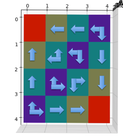
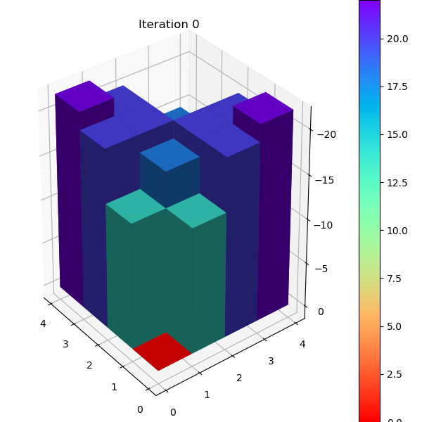
V = np.zeros(env.nS)
changed_state_set = set(s for s in range(env.nS))

iter = 0
while len(changed_state_set) > 0:
changed_state_set_ = set()
for s in changed_state_set:
action_values = action_value(env, s, V, gamma=gamma)
best_action_value = np.max(action_values)
v_diff = np.abs(best_action_value - V[s])
if v_diff > theta:
changed_state_set_.update(mapping[s])
V[s] = best_action_value
changed_state_set = changed_state_set_
iter += 1

policy = np.zeros([env.nS, env.nA])
for s in range(env.nS):
action_values = action_value(env, s, V, gamma=gamma)
best_action = np.argmax(action_values)
policy[s, best_action] = 1.0

return policy, V
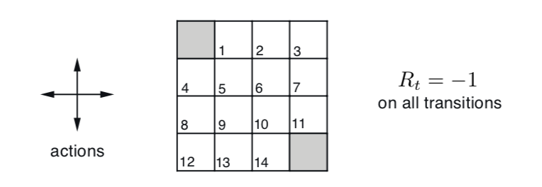
比较值迭代和异步值迭代方法后发现,值迭代用了4次循环,每次涉及所有状态,总计算状态数为 4 x 16 = 64。异步值迭代也用了4次循环,但是总计更新了54个状态。由于Grid World 的状态数很少,异步值迭代优势并不明显,但是对于状态数众多并且迭代最终集中在少部分状态的环境下,节省的计算量还是很可观的。

Your browser is out-of-date!

Update your browser to view this website correctly. Update my browser now

×