NeuralProphet深度学习版Prophet
NeuralProphet 负有盛名,是 Facebook开发的新一代 Prophet
时间序列预测框架,堪称时间序列预测神器。但是它的API使用,调参,原理不太为大家所知,我们会花几期文章和视频,我们将由浅入深,由实践至原理,揭开其神秘面纱。
NeuralProphet 继承了 Prophet
模块可接受性的特点,将预测的值分解到趋势、季节性、AR、事件(节日)几个模块。其中
AR 部分的神经网络实现由 AR-Net: A simple Auto-Regressive Neural
Network for time-series 这篇论文详细描述。此外,NeuralProphet
整体用 PyTorch 重新实现,主要特性如下
- 使用 PyTorch 的优化,性能比原始 Prophet 快不少
- 引入 AR-Net 建模时间序列自回归,并配有非线性层
- 自定义损失和指标
- 滞后协变量(lagged covariates) 和 AR 本地上下文特性 (local context)
尽管 NeuralProphet
有不少优势,但是使用起来小问题不断,主要表现为文档不甚详细,API
设计的比较智能(隐晦),坑不少。这一期我们来实战体验一下,后续会深入代码和论文。
相关论文链接:
[Prophet] Forecasting at scale https://peerj.com/preprints/3190/
NeuralProphet: Explainable Forecasting at Scale https://arxiv.org/abs/2111.15397
AR-Net: A simple Auto-Regressive Neural Network for time-series https://arxiv.org/abs/1911.12436
安装NeuralProphet
使用命令通过 pip 就可以安装 NeuralProphet。
1 | pip install neuralprophet==0.5.0 |
如果在 Jupyter Notebook 中使用 NeuralProphet,最好安装实时版本,允许你实时可视化模型损失。
1 | pip install neuralprophet[live]==0.5.0 |
要注意一点,安装 neuralprophet 会关联安装 Pytorch CPU版本库,如果你需要使用 GPU 或者不希望覆盖原有的 Pytorch 版本,请手动安装。
此外,MyEncyclopedia 和往常一样,为大家准备了一个 docker 镜像,预装最新的 NeuralProphet 库,镜像中还包含预下载的数据集和本文所有的 Jupyter Notebook 代码。大家关注 MyEncyclopedia公众号,执行下面命令后网页打开 http://localhost:8888/ 开箱即用
1 | docker pull myencyclopedia/neuralprophet-tut |
标准普尔 500 指数数据集
这次实战我们使用过去 10 年标准普尔 500 指数的每日股价数据。可以通过如下命令下载数据集,使用 docker 镜像的同学无需额外下载。
1 | import pandas_datareader as pdr |
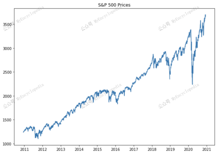
从图中我们可以清楚地看到标准普尔 500 指数总体呈上升趋势,其中有几个点的价格大幅上涨或下跌。我们可以将这些点视为趋势变化点。鉴于此,我们先从一个仅有趋势模块的 NeuralProphet 模型开始,逐渐加入季节性,AR和节日模块,观察其预测表现和API 具体使用。
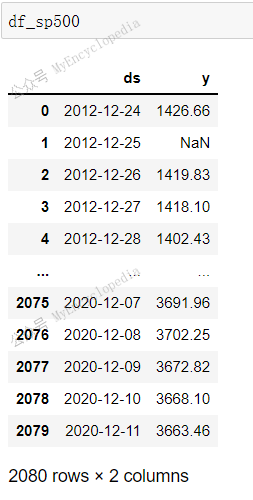
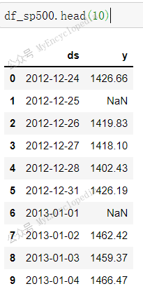
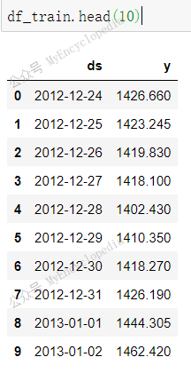
使用 NeuralProphet,我们必须确保数据的格式包含如下两列:日期列名ds,目标变量列名 y。
1 | df_sp500 = df_sp500.reset_index().rename(columns={'DATE': 'ds', 'sp500': 'y'}) |
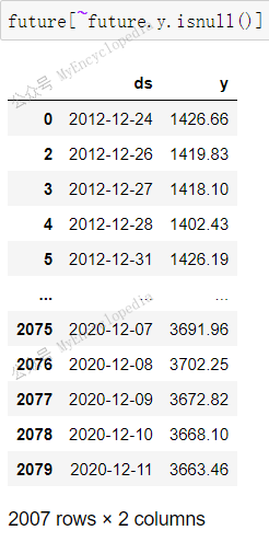
1 | len(df_sp500[~df_sp500.y.isnull()]) |
总结 SP 500 数据观察到的特点,后面会反复和过程变量做对比:
总共2080条数据中非空数据有2007条
开始日期为 2012-12-24,结束日期 2020-12-11
在上述有效时间段内,非交易的日期(周末,节日)没有在列。
模块一:趋势
使用 NeuralProphet,我们可以通过指定几个重要参数来对时间序列数据中的趋势进行建模。
- n_changepoints — 指定趋势发生变化的点数。
- trend_reg — 控制趋势变化点的正则化参数。较大的值 (~1–100) 将惩罚更多的变化点。较小的值 (~0.001–1.0) 将允许更多的变化点。
- changepoints_range — 默认值 0.8,表示后20%的训练数据无 changepoints
1 | model = NeuralProphet(n_changepoints=100, |
训练模型
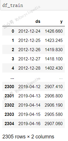
1 | df_train, df_val = model.split_df(df_sp500, freq="D", valid_p=0.2) |
1 | metrics = model.fit(df_train, |
训练最终趋于稳定。我们来看看 split_df API 的细节。
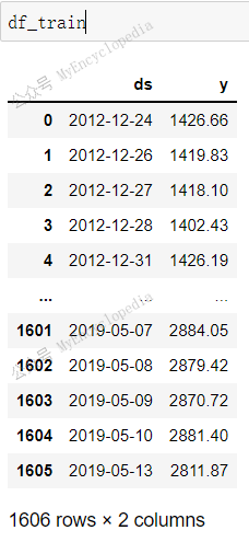
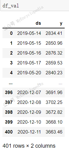
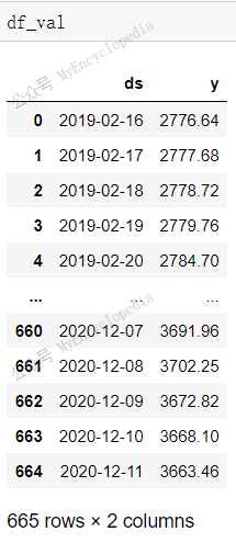
df_train 共1606 行,为前 80% 记录,df_val
共401 行,为后20% 记录,两者没有交集,合计 2007 行数据,等于
df_sp500 有效数据数。原来默认情况下 split_df
会扔掉 y 值为 NaN
数据。这里两者没有交集,大家注意对比启用AR后的数据切分两者会有交集。原有是启用自回归后,预测需要过去
k 个点作为输入。
预测验证集
接着来看看验证集,即 df_val 上的预测表现。
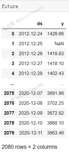
1 | future = model.make_future_dataframe(df_sp500, periods=60, n_historic_predictions=True) |
make_future_dataframe 准备好待预测的数据格式,参数
periods=60,n_historic_predictions=True
意义扩展 df_sp500 到未来60天后,同时保留所有所有现有
df_sp500 的数据点,这些历史点也将做预测。我们 dump 出
make_future_dataframe 后的 future 变量。
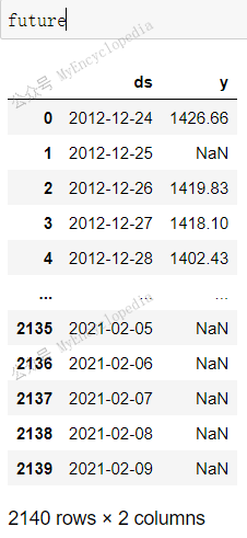
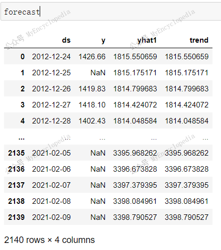
future 序列扩展了 df_sp500,有 y
值的共2007条,和 df_sp500 一致。时间扩展到了
2021-02-09,大约是 2021-12-11 后的60天,这个也和总条数 2140 一致,等于
df_sp500 总条数 2080 加上 periods=60
的部分。
接着来看 predict 后的 forecast 变量。y 列依然有 2007
条,多了 yhat1 和 trend 两列。
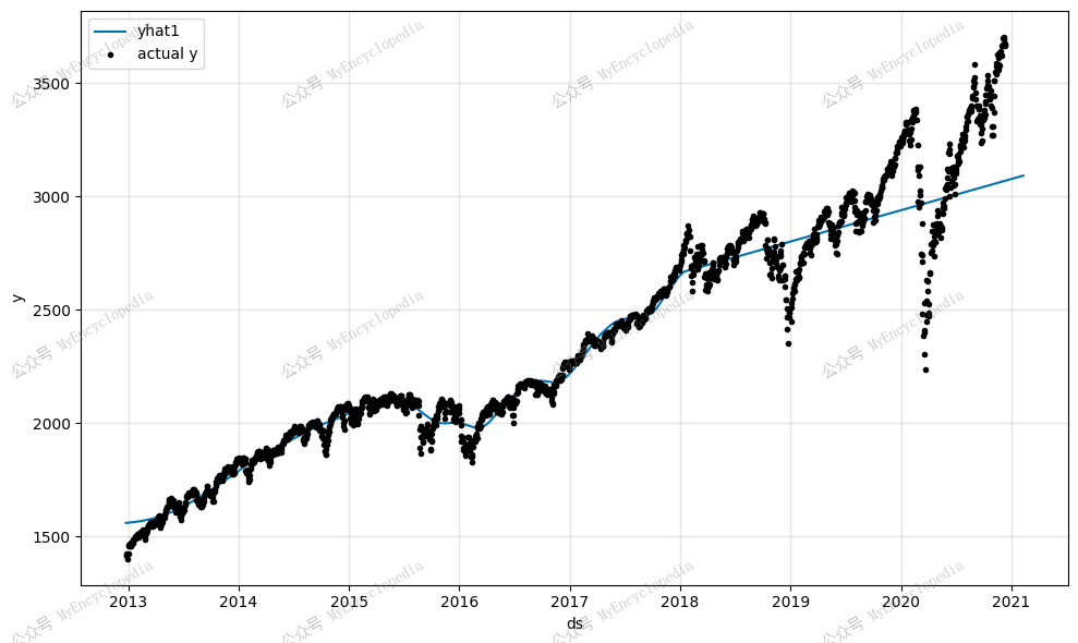
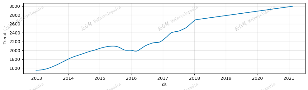
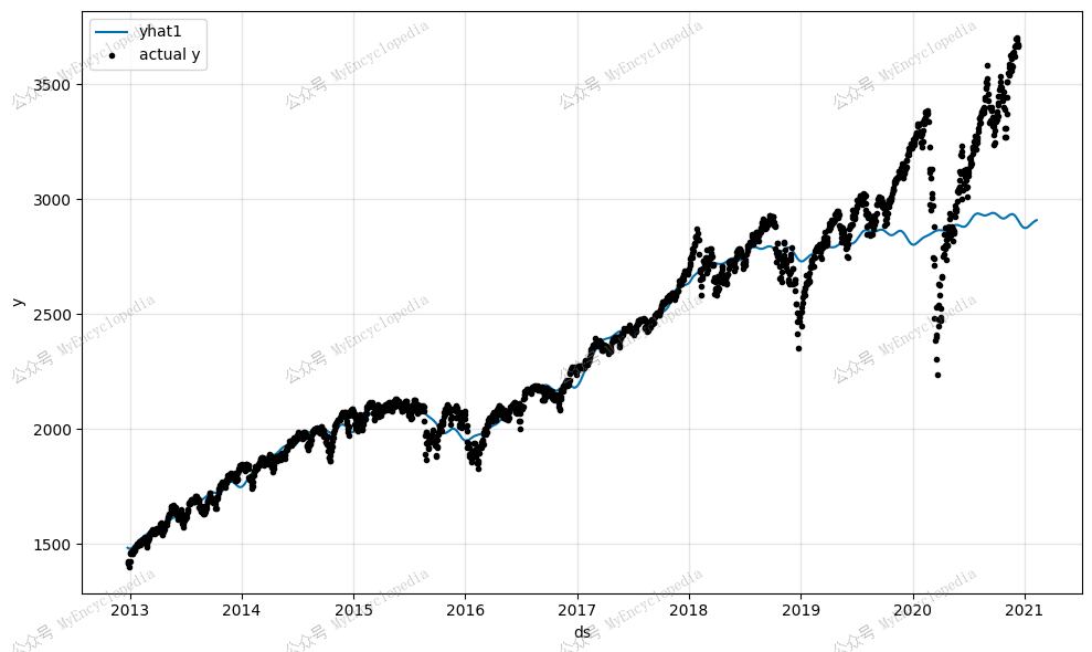
最后,model.plot(forecast)
会绘制出事实点和预测点的曲线,注意图中预测值比实际值要稍长一些,因为预测值到
2021-02-09,实际值仅到
2020-12-11。
模块归因
1 | fig_components = model.plot_components(forecast) |
由于只启用了趋势,只有一个模块输出。
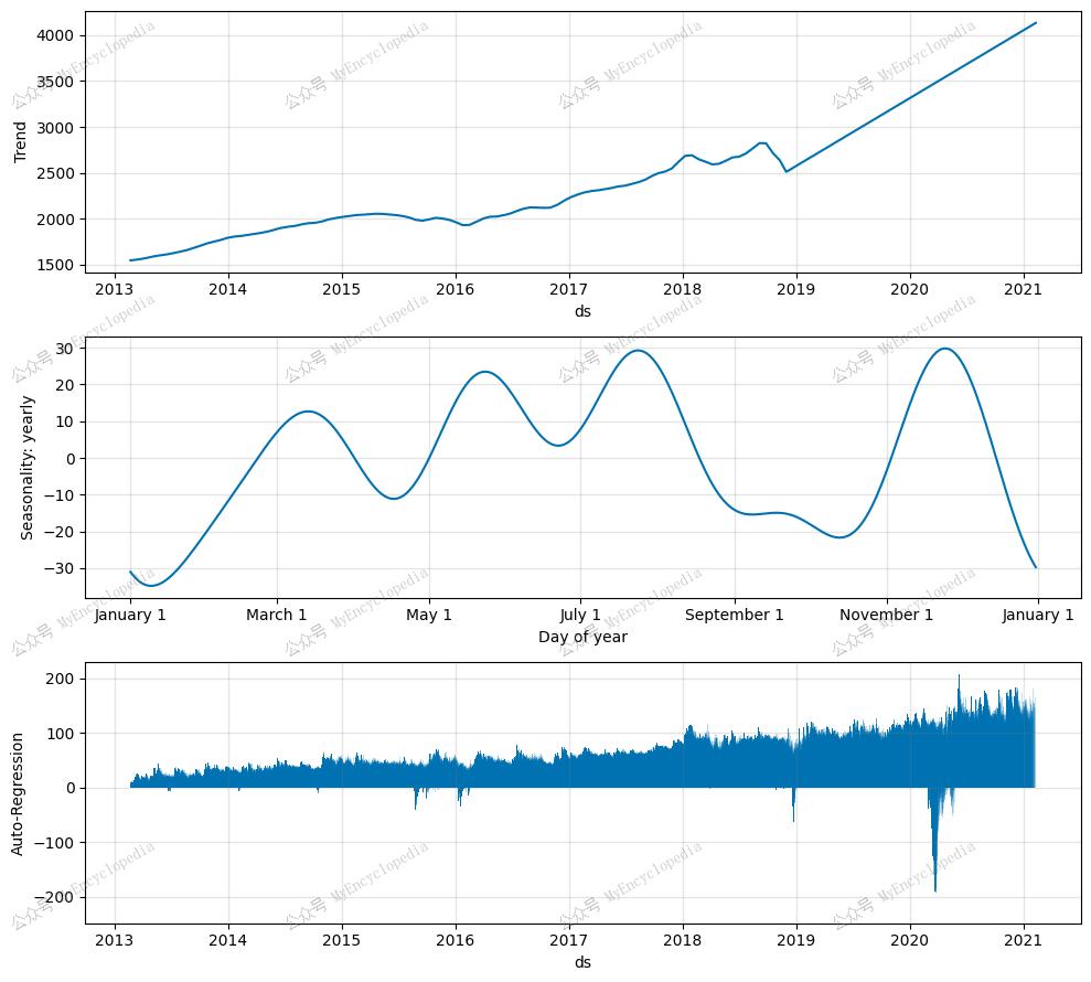
很明显,我们的模型捕捉到了标准普尔 500 指数的总体上涨趋势,但该模型存在欠拟合问题,尤其是当我们查看未知未来的60天的预测,更能发现问题。
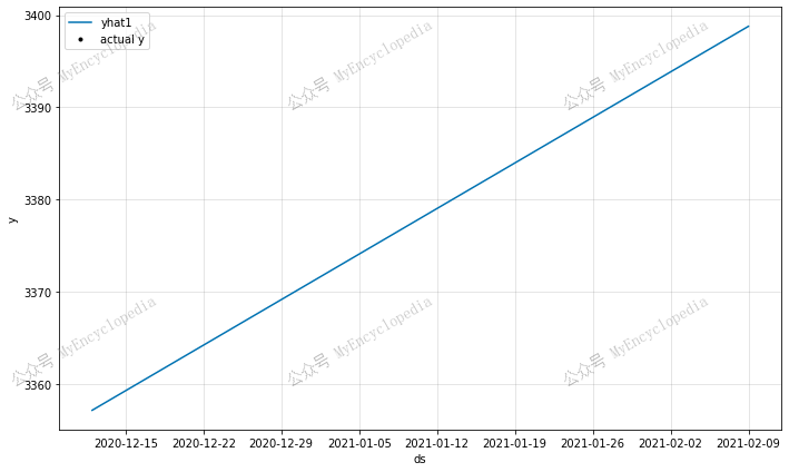
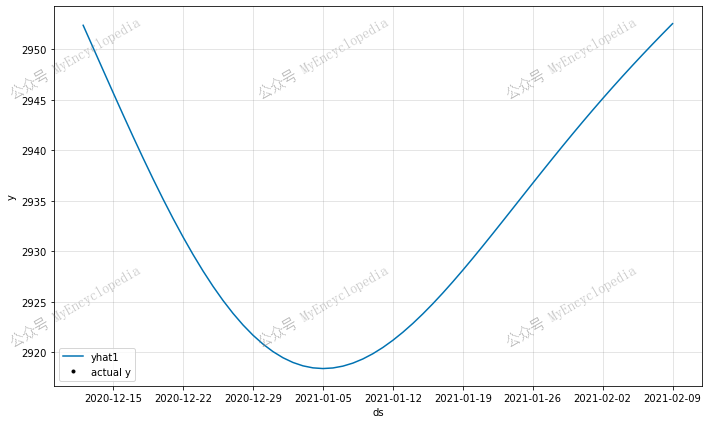
仅预测未来
同样的预测代码,将n_historic_predictions 改成 False
会只预测未知未来60天。
1 | future = model.make_future_dataframe(df_sp500, periods=60, n_historic_predictions=False) |
1 | print(len(future), len(forecast)) |
根据上图,我们可以看到模型对未来的预测遵循一条直线,天天上涨的股票,还在这里看什么,还不赶紧去买!
模块二:季节性
真实世界的时间序列数据通常涉及季节性模式。即使对于股票市场也是如此,一月效应等趋势可能会逐年出现。我们可以通过添加年度季节性来使之前的模型更加完善。
1 | model = NeuralProphet(n_changepoints=100, |
预测验证集
和之前一条直线相比,现在对数据的预测显得更现实些。
模块归因
现在预测的 Y 值是两个部分的模块的加和了。
1 | fig_components = model.plot_components(forecast) |
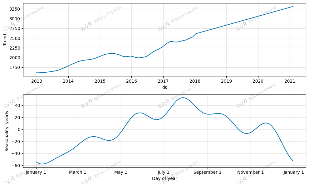
标准普尔 500 指数预测具有年度季节性,包括历史数据。
仅预测未来
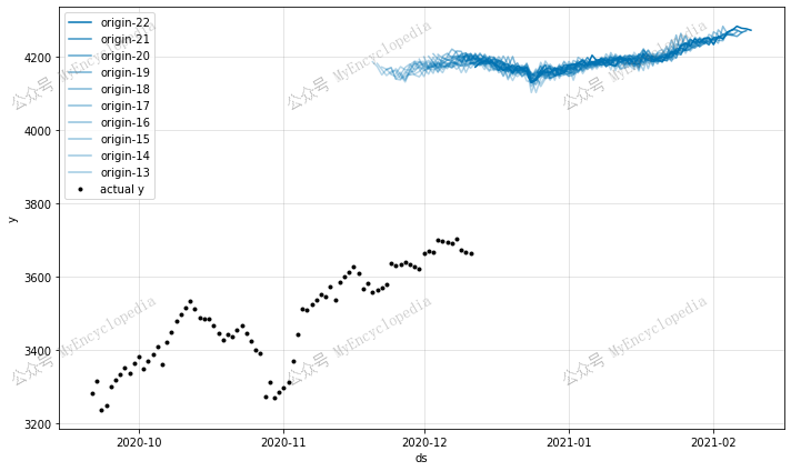
1 | plot_forecast(model, sp500_data, periods=60, historic_predictions=False, highlight_steps_ahead=60) |
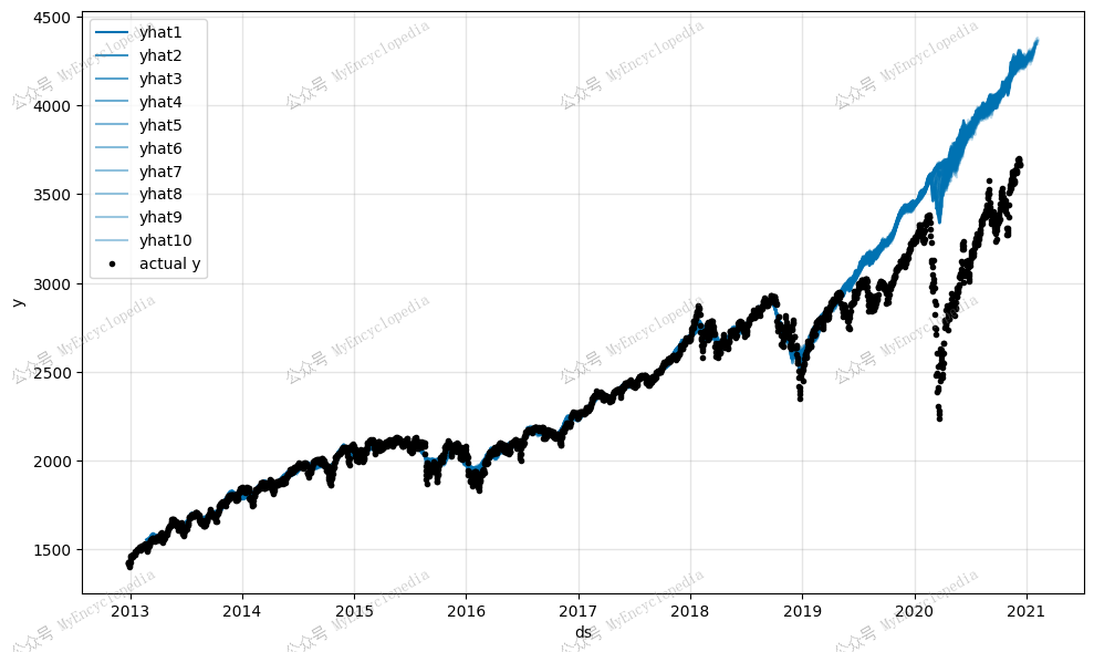
根据上图,我们可以看到这个模型更真实一些,但仍然存在欠拟合问题。因此,我们再引入自回归模型 AR 来进一步拟合。
模块三:自回归 AR
AR-Net 是一种用于时间序列预测的自回归神经网络。自回归模型使用来自过去历史数据点来预测后续点,这就是自回归一词的来源。
例如,为了预测标准普尔 500 指数的价格,我们可以训练一个模型,使用过去 60 天的价格来预测未来 60 天的价格。分别对应以下代码中的n_lags和n_forecasts参数。
1 | model = NeuralProphet( |
训练模型
1 | df_train, df_val = model.split_df(df_sp500, freq="D", valid_p=0.2) |
切分训练和验证集代码一样,但是由于引入
AR,df_train,df_val
之间有60条数据重合,这是因为,在验证或者预测过程中,传入的 dataframe
前60条不做预测,从61条开始预测,预测会使用当前日期前60条作为 AR
模块的输入。
1 | len(set(df_train.ds.tolist()).intersection(set(df_val.ds.tolist()))) |
不过奇怪的是,df_train 加上 df_val 总共有
2305 + 665 = 2970 条记录,时间跨度依然是 2012-12-24 至
2020-12-11。但是去除重复的60条记录后居然剩余2910 条, 比
df_sp500 2080 条记录数还要多不少。
这里笔者稍微花了点时间终于弄清楚:df_train 和
df_val 会填充 2012-12-24 至 2020-12-11 所有的 missing
日期,并使用插值填充 y!
预测验证集
这一次,我们将 periods 设成 0,也就是不扩展
df_sp500 时间到未知的未来。
1 | future = model.make_future_dataframe(df_sp500, periods=0, n_historic_predictions=True) |
1 | forecast = model.predict(future) |
forecast 格式变得复杂,引入了 yhat1, yhat2,
...,yhat60,ar1, ar2, ...,ar60 等众多列,这里的60对应于
n_forecasts=60
第一个预测值开始于 forecast 的第61条记录,对应于
n_lags = 60
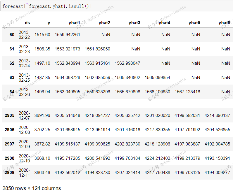
1 | forecast[~forecast.yhat1.isnull()] |
1 | fig = model.plot(forecast) |
模块归因
1 | fig_components = model.plot_components(forecast) |
仅预测未来
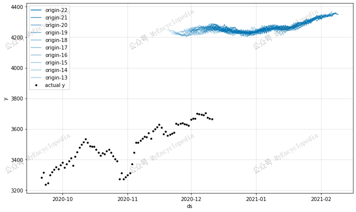
1 | future = model.make_future_dataframe(df_sp500, periods=60, n_historic_predictions=False) |
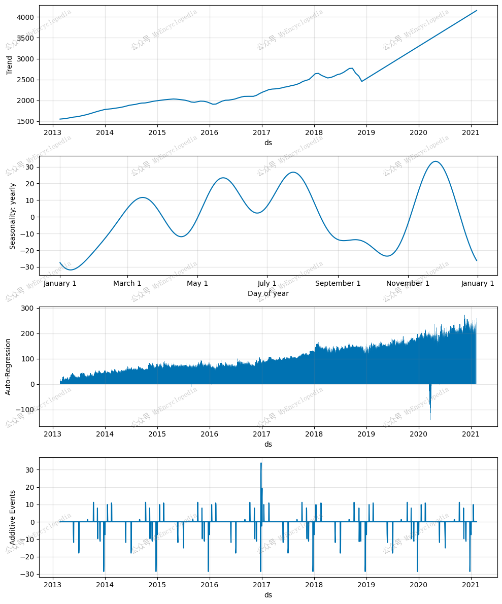
模块四:事件(节日)
我们还可以配置模型以考虑节假日因素,因为节假日很可能会影响股市走势。
1 | model = NeuralProphet( |
只需 add_country_holidays
一条语句就可以启用预定义的美国节假日。
1 | plot_forecast(model, sp500_data, periods=60, historic_predictions=False, highlight_steps_ahead=60) |
预测验证集

模块归因
1 | fig_components = model.plot_components(forecast) |
仅预测未来
1 | future = model.make_future_dataframe(df_sp500, periods=60, n_historic_predictions=False) |