从零构建统计随机变量生成器之离散基础篇

在本系列中，我们会从第一性原理出发，从零开始构建统计学中的常见分布的随机变量生成器，包括二项分布，泊松分布，高斯分布等。在实现这些基础常见分布的过程中，会展示如何使用统计模拟的通用技术，包括 inverse CDF，Box-Muller，分布转换等。本期通过伯努利试验串联起来基础离散分布并通过代码来实现这些分布的生成函数，从零开始构建的原则是随机变量生成器实现只依赖 random() 产生 [0, 1.0] 之间的浮点数，不依赖于其他第三方API来完成。

• 从零构建统计随机变量生成器之 离散基础篇
• 从零构建统计随机变量生成器之 用逆变换采样方法构建随机变量生成器
• 深入 LeetCode 470 拒绝采样，状态转移图求期望和一道经典统计求期望题目
• 从零构建统计随机变量生成器之 正态分布 Box-Muller方法

均匀分布（离散）

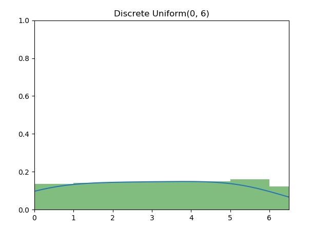
离散均匀分布（Discrete Uniform Distribution）的随机变量是最为基本的，图中为 [0, 6] 七个整数的离散均匀分布。算法实现为，使用 [0, 1] 之间的随机数 u，再将 u 等比例扩展到指定的整数上下界。

实现代码

import random
from math import floor

def uniform(a: int, b: int) -> int:
    assert a <= b
    u = random.random()
    return a + floor((b - a + 1) * u)

Github 代码地址：

https://github.com/MyEncyclopedia/stats_simulation/blob/main/distrib_sim/discrete_uniform.py

伯努利分布

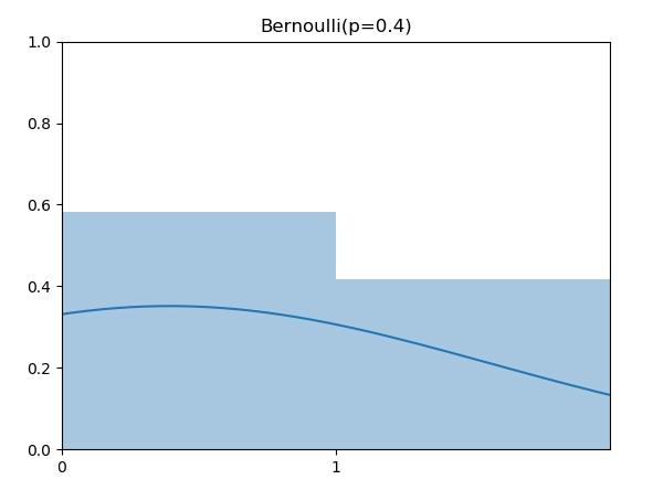
伯努利分布（Bernoulli Distribution）是support为0或者1的离散分布，0和1可以看成失败和成功两种可能。伯努利分布指定了成功的概率p，例如，下图是 p=0.4 的伯努利分布。

伯努利分布随机数实现也很直接，将随机值 u 根据 p 决定成功或者失败。

实现代码

import random

def bernoulli(p: float) -> int:
    assert 0 <= p <= 1
    u = random.random()
    return 1 if u <= p else 0

Github 代码地址：

https://github.com/MyEncyclopedia/stats_simulation/blob/main/distrib_sim/discrete_bernoulli.py

类别分布

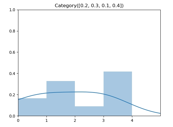
类别分布（Categorical Distribution）是在伯努利分布的基础上扩展到了多个点，每个点同样由参数指定了其概率，因此，其参数从 p 扩展到了向量 \(\vec p\)，如图所示为 $p = [0.2, 0.3, 0.1, 0.4] $ 时的类别分布。

实现代码

类别分布生成函数也扩展了伯努利分布的实现算法，将随机数 u 和累计概率向量作比较。在这个例子中， $p = [0.2, 0.3, 0.1, 0.4] $ 转换成 $c = [0.2, 0.5, 0.6, 1] $，再将 u 和 \(\vec c\)数组匹配，返回结果为第一个大于 u 的元素 index。实现上，我们可以以线性复杂度遍历数组，更好一点的方法是，用 python bisect函数通过二分法找到index，将时间复杂度降到 \(O(log(n))\)。

import bisect
import random
from typing import List

def categorical(probs: List[float]) -> int:
    assert abs(sum(probs) - 1.0) < 0.001
    cum = probs.copy()

    for i in range(1, len(cum)):
        cum[i] = cum[i-1] + probs[i]

    u = random.random()
    return bisect.bisect(cum, u)

Github 代码地址： https://github.com/MyEncyclopedia/stats_simulation/blob/main/distrib_sim/discrete_categorical.py

二项分布

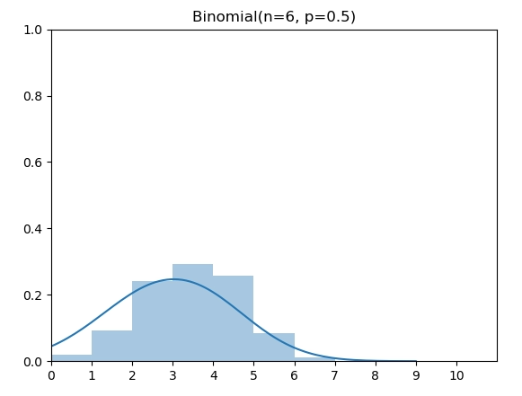
二项分布（Binomial Distribution）有两个参数 n 和 p，表示伯努利实验做n次后成功的次数。图中为 n=6，p=0.5的二项分布。

实现代码

二项分布生成算法可以通过伯努利试验的故事来实现，即调用 n 次伯努利分布生成函数，返回总的成功次数。

def binomial(n: int, p: float) -> int:
    return sum(bernoulli(p) for _ in range(n))

Github 代码地址：

https://github.com/MyEncyclopedia/stats_simulation/blob/main/distrib_sim/discrete_binomial.py

概率质量函数（PMF）

\[ \operatorname{Pr}_\text{Binomial}(X=k)=\left(\begin{array}{c}n \\ k\end{array}\right)p^{k}(1- p)^{n-k} \]

几何分布

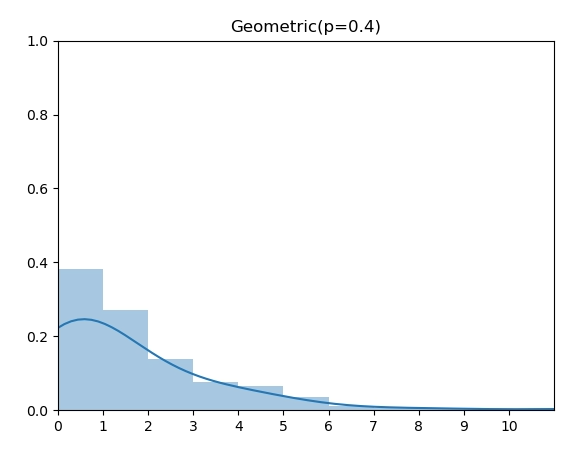
几何分布（Geometric Distribution）和伯努利实验的关系是：几何分布是反复伯努利实验直至第一次成功时的失败次数。如图，当成功概率 p=0.4时的几何分布。

实现代码

from discrete_bernoulli import bernoulli

def geometric(p: float) -> int:
    fail_num = 0
    while not bernoulli(p):
        fail_num += 1
    return fail_num

Github 代码地址：

https://github.com/MyEncyclopedia/stats_simulation/blob/main/distrib_sim/discrete_geometric.py

概率质量函数（PMF）

\[ \operatorname{Pr}_\text{Geometric}(X=k)=(1-p)^{k-1} p \]

负二项分布

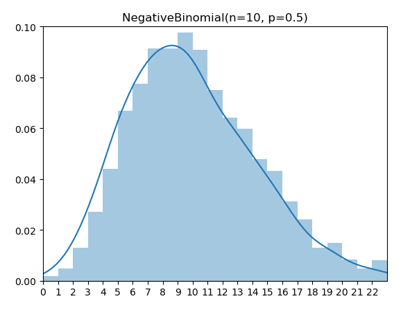
负二项分布（Negative Binomial Distribution）是尝试伯努利试验直至成功 r 次的失败次数。

实现代码

from discrete_bernoulli import bernoulli

def negative_binomial(r: int, p: float) -> int:
    failures = 0
    while r:
        success = bernoulli(p)
        if success:
            r -= 1
        else:
            failures += 1
    return failures

Github 代码地址：

https://github.com/MyEncyclopedia/stats_simulation/blob/main/distrib_sim/discrete_nagative_binomial.py

概率质量函数（PMF）

\[ \operatorname{Pr}_\text{NegBinomial}(X=k)=\left(\begin{array}{c}k+r-1 \\ r-1\end{array}\right)(1-p)^{k} p^{r} \]

超几何分布

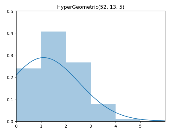
超几何分布（HyperGeometric Distribution）的意义是从总数为N的集合抽取n次后成功的次数。具体来说，集合由K个表示成功的元素和N-K个表示失败的元素组成，并且抽取时没有替换（without replacement）情况下的成功次数。注意，超几何分布和二项分布的区别仅在于有无替换。

实现代码

from discrete_bernoulli import bernoulli

def hypergeometric(N: int, K_succ_num: int, n_trial_num: int) -> int:
    x = N - K_succ_num
    n_hit = 0
    while n_trial_num:
        hit = bernoulli(K_succ_num / (K_succ_num + x))
        n_hit += hit
        if hit:
            K_succ_num -= 1
        else:
            x -= 1
        if K_succ_num == 0:
            return n_hit
        n_trial_num -= 1
    return n_hit

Github 代码地址：

https://github.com/MyEncyclopedia/stats_simulation/blob/main/distrib_sim/discrete_hypergeometric.py

概率质量函数（PMF）

\[ \operatorname{Pr}_\text{Hypergeo}(X=k)=\frac{\left(\begin{array}{c}K \\ k\end{array}\right)\left(\begin{array}{c}N-k \\ n-k\end{array}\right)}{\left(\begin{array}{l}N \\ n\end{array}\right)} \]

负超几何分布

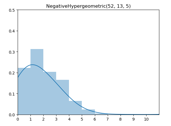
负超几何分布（Negative Hypergeometric Distribution）的意义是从总数为N的集合中，无替换下抽取直至 r 次失败时，成功的次数。

实现代码

from discrete_bernoulli import bernoulli

def negative_hypergeometric(N: int, K_success_num: int, r_fail_times: int) -> int:
    fail_num = N - K_success_num
    succ_trials = 0
    while r_fail_times:
        success = bernoulli(K_success_num / (K_success_num + fail_num))
        if success:
            K_success_num -= 1
            succ_trials += 1
            if K_success_num == 0: # no more success elements
                return succ_trials
        else:
            fail_num -= 1
            r_fail_times -= 1
    return succ_trials

Github 代码地址： https://github.com/MyEncyclopedia/stats_simulation/blob/main/distrib_sim/discrete_negative_hypergeometric.py

概率质量函数（PMF）

\[ \operatorname{Pr}_\text{NegHypergeo}(X=k)=\frac{\left(\begin{array}{c}k+r-1 \\ k\end{array}\right)\left(\begin{array}{c}N-r-k \\ K-k\end{array}\right)}{\left(\begin{array}{l}N \\ K\end{array}\right)} \quad \text{for } k=0,1,2, \ldots, K \]

伯努利试验总结

下表总结了上面四种和伯努利试验有关的离散分布的具体区别。

	有替换	无替换
固定尝试次数	二项 Binomial	超几何 Hypergeometric
固定成功次数	负二项 Negative Binomial	负超几何 Negative Hypergeometric