通过代码学Sutton强化学习2：Grid World 策略迭代和值迭代

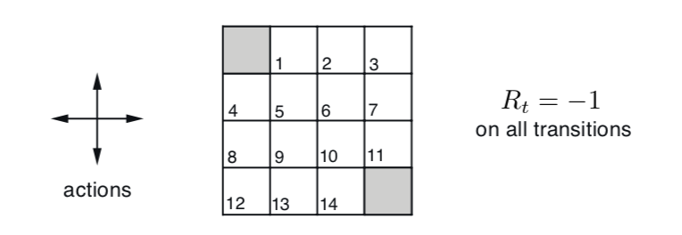
上一期 通过代码学Sutton强化学习1：Grid World OpenAI环境和策略评价算法，我们引入了 Grid World 问题，实现了对应的OpenAI Gym 环境，也分析了其最佳策略和对应的V值。这一期中，继续通过这个例子详细讲解策略提升（Policy Improvment）、策略迭代（Policy Iteration）、值迭代（Value Iteration）和异步迭代方法。

回顾 Grid World 问题

Grid World 问题

在Grid World 中，Agent初始可以出现在编号1-14的网格中，Agent 每往四周走一步得到 -1 reward，因此需要尽快走到两个出口。当然最佳策略是以最小步数往出口逃离，如下所示。

Grid World 最佳策略

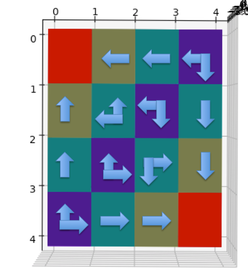
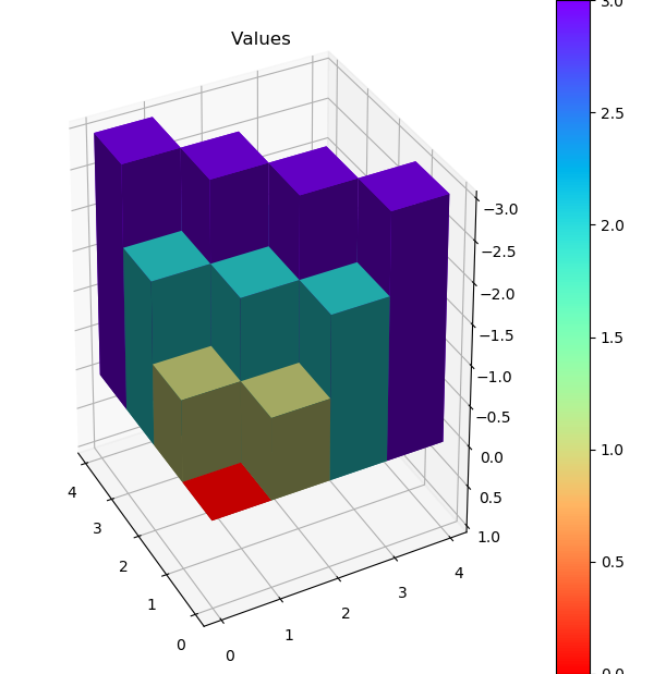
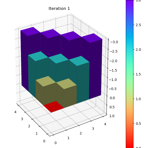
最佳策略对应的状态V值和3D heatmap如下

[[ 0. -1. -2. -3.]
 [-1. -2. -3. -2.]
 [-2. -3. -2. -1.]
 [-3. -2. -1.  0.]]

Grid World V值 3D heatmap

策略迭代

上一篇中，我们知道如何evaluate 给定policy \(\pi\) 的 \(v_{\pi}\)值，那么是否可能在此基础上改进生成更好的策略 \(\pi^{\prime}\)。如果可以，能否最终找到最佳策略\({\pi}_{*}\)？答案是肯定的，因为存在策略提升定理（Policy Improvement Theorem）。

策略提升定理

在 4.2 节 Policy Improvement Theorem 可以证明，利用 \(v_{\pi}\) 信息对于每个状态采取最 greedy 的 action （又称exploitation）能够保证生成的新 \({\pi}^{\prime}\) 是不差于旧的policy \({\pi}\)，即

\[ q_{\pi}(s, {\pi}^{\prime}(s)) \gt v_{\pi}(s) \]

\[ v_{\pi^{\prime}}(s) \gt v_{\pi}(s) \]

因此，可以通过在当前policy求得v值，再选取最greedy action的方式形成如下迭代，就能够不断逼近最佳策略。

\[ \pi_{0} \stackrel{\mathrm{E}}{\longrightarrow} v_{\pi_{0}} \stackrel{\mathrm{I}}{\longrightarrow} \pi_{1} \stackrel{\mathrm{E}}{\longrightarrow} v_{\pi_{1}} \stackrel{\mathrm{I}}{\longrightarrow} \pi_{2} \stackrel{\mathrm{E}}{\longrightarrow} \cdots \stackrel{\mathrm{I}}{\longrightarrow} \pi_{*} \stackrel{\mathrm{E}}{\longrightarrow} v_{*} \]

策略迭代算法

以下为书中4.3的policy iteration伪代码。其中policy evaluation的算法在上一篇中已经实现。Policy improvement 的精髓在于一次遍历所有状态后，通过policy 的最大Q值找到该状态的最佳action，并更新成最新policy，循环直至没有 action 变更。

\[ \begin{align*} &\textbf{Policy Iteration (using iterative policy evaluation) for estimating } \pi\approx {\pi}_{*} \\ &1. \quad \text{Initialization} \\ & \quad \quad V(s) \in \mathbb R\text{ and } \pi(s) \in \mathcal A(s) \text{ arbitrarily for all }s \in \mathcal{S} \\ & \\ &2. \quad \text{Policy Evaluation} \\ & \quad \quad \text{Loop:}\\ & \quad \quad \Delta \leftarrow 0\\ & \quad \quad \text{Loop for each } s \in \mathcal{S}:\\ & \quad \quad \quad \quad v \leftarrow V(s) \\ & \quad \quad \quad \quad V(s) \leftarrow \sum_{s^{\prime}, r} p\left(s^{\prime}, r \mid s, a\right)\left[r+\gamma V\left(s^{\prime}\right)\right] \\ & \quad \quad \quad \quad \Delta \leftarrow \max(\Delta, |v-V(s)|) \\ & \quad \quad \text{until } \Delta < \theta \text{ (a small positive number determining the accuracy of estimation)}\\ & \\ &3. \quad \text{Policy Improvement} \\ & \quad \quad policy\text{-}stable\leftarrow true \\ & \quad \quad \text{Loop for each } s \in \mathcal{S}:\\ & \quad \quad \quad \quad old\text{-}action\leftarrow \pi(s) \\ & \quad \quad \quad \quad \pi(s) \leftarrow \operatorname{argmax}_{a} \sum_{s^{\prime}, r} p\left(s^{\prime}, r \mid s, a\right)\left[r+\gamma V\left(s^{\prime}\right)\right] \\ & \quad \quad \quad \quad \text{If } old\text{-}action \neq \pi\text{,then }policy\text{-}stable\leftarrow false \\ & \quad \quad \text{If } policy\text{-}stable \text{, then stop and return }V \approx v_{*} \text{ and } \pi\approx {\pi}_{*}\text{; else go to 2} \end{align*} \]

注意到状态Q值 \(q_{\pi}(s, a)\) 会被多处调用，将其封装为单独的函数。

\[ \begin{aligned} q_{\pi}(s, a) &=\sum_{s^{\prime}, r} p\left(s^{\prime}, r \mid s, a\right)\left[r+\gamma v_{\pi}\left(s^{\prime}\right)\right] \end{aligned} \]

Q值函数实现如下：

{linenos

def action_value(env: GridWorldEnv, state: State, V: StateValue, gamma=1.0) -> ActionValue:
    q = np.zeros(env.nA)
    for a in range(env.nA):
        for prob, next_state, reward, done in env.P[state][a]:
            q[a] += prob * (reward + gamma * V[next_state])
    return q

有了 action_value 和上期的 policy_evaluate，policy iteration 实现完全对应上面的伪代码。

{linenos

def policy_improvement(env: GridWorldEnv, policy: Policy, V: StateValue, gamma=1.0) -> bool:
    policy_stable = True

    for s in range(env.nS):
        old_action = np.argmax(policy[s])
        Q_s = action_value(env, s, V)
        best_action = np.argmax(Q_s)
        policy[s] = np.eye(env.nA)[best_action]

        if old_action != best_action:
            policy_stable = False
    return policy_stable


def policy_iteration(env: GridWorldEnv, policy: Policy, gamma=1.0) -> Tuple[Policy, StateValue]:
    iter = 0
    while True:
        V = policy_evaluate(policy, env, gamma)
        policy_stable = policy_improvement(env, policy, V)
        iter += 1

        if policy_stable:
            return policy, V

Grid World 例子通过两轮迭代就可以收敛，以下是初始时随机策略的V值和第一次迭代后的V值。

初始随机策略 V 值

第一次迭代后的 V 值

值迭代

值迭代（ Value Iteration）的本质是，将policy iteration中的policy evaluation过程从不断循环到收敛直至小于theta，改成只执行一遍，并直接用最佳Q值更新到状态V值，如此可以不用显示地算出\({\pi}\) 而直接在V值上迭代。具体迭代公式如下：

\[ \begin{aligned} v_{k+1}(s) & \doteq \max _{a} \mathbb{E}\left[R_{t+1}+\gamma v_{k}\left(S_{t+1}\right) \mid S_{t}=s, A_{t}=a\right] \\ &=\max_{a} q_{\pi_k}(s, a) \\ &=\max _{a} \sum_{s^{\prime}, r} p\left(s^{\prime}, r \mid s, a\right)\left[r+\gamma v_{k}\left(s^{\prime}\right)\right] \end{aligned} \]

完整的伪代码为：

\[ \begin{align*} &\textbf{Value Iteration, for estimating } \pi\approx \pi_{*} \\ & \text{Algorithm parameter: a small threshold } \theta > 0 \text{ determining accuracy of estimation} \\ & \text{Initialize } V(s), \text{for all } s \in \mathcal{S}^{+} \text{, arbitrarily except that } V (terminal) = 0\\ & \\ &1: \text{Loop:}\\ &2: \quad \quad \Delta \leftarrow 0\\ &3: \quad \quad \text{Loop for each } s \in \mathcal{S}:\\ &4: \quad \quad \quad \quad v \leftarrow V(s) \\ &5: \quad \quad \quad \quad V(s) \leftarrow \operatorname{max}_{a} \sum_{s^{\prime}, r} p\left(s^{\prime}, r \mid s, a\right)\left[r+\gamma V\left(s^{\prime}\right)\right] \\ &6: \quad \quad \quad \quad \Delta \leftarrow \max(\Delta, |v-V(s)|) \\ &7: \text{until } \Delta < \theta \\ & \\ & \text{Output a deterministic policy, }\pi\approx \pi_{*} \text{, such that} \\ & \quad \quad \pi(s) \leftarrow \operatorname{argmax}_{a} \sum_{s^{\prime}, r} p\left(s^{\prime}, r \mid s, a\right)\left[r+\gamma V\left(s^{\prime}\right)\right] \end{align*} \]

代码实现也比较直接，可以复用上面已经实现的 action_value 函数。

{linenos

def value_iteration(env:GridWorldEnv, gamma=1.0, theta=0.0001) -> Tuple[Policy, StateValue]:
    V = np.zeros(env.nS)
    while True:
        delta = 0
        for s in range(env.nS):
            action_values = action_value(env, s, V, gamma=gamma)
            best_action_value = np.max(action_values)
            delta = max(delta, np.abs(best_action_value - V[s]))
            V[s] = best_action_value
        if delta < theta:
            break

    policy = np.zeros([env.nS, env.nA])
    for s in range(env.nS):
        action_values = action_value(env, s, V, gamma=gamma)
        best_action = np.argmax(action_values)
        policy[s, best_action] = 1.0

    return policy, V

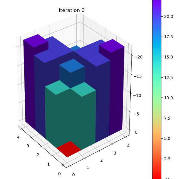
异步迭代

在第4.5节中提到了DP迭代方式的改进版：异步方式迭代（Asychronous Iteration）。这里的异步是指每一轮无需全部扫一遍所有状态，而是根据上一轮变化的状态决定下一轮需要最多计算的状态数，类似于Dijkstra最短路径算法中用 heap 来维护更新节点集合，减少运算量。下面我们通过异步值迭代来演示异步迭代的工作方式。

下图表示状态的变化方向，若上一轮 \(V(s)\) 发生更新，那么下一轮就要考虑状态 s 可能会影响到上游状态的集合（ p1，p2），避免下一轮必须遍历所有状态的V值计算。

Async 反向传播

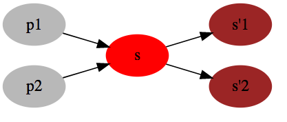
要做到部分更新就必须知道每个状态可能影响到的上游状态集合，上图对应的映射关系可以表示为

\[ \begin{align*} s'_1 &\rightarrow \{s\} \\ s'_2 &\rightarrow \{s\} \\ s &\rightarrow \{p_1, p_2\} \end{align*} \]

建立映射关系的代码如下，build_reverse_mapping 返回类型为 Dict[State, Set[State]]。

{linenos

def build_reverse_mapping(env:GridWorldEnv) -> Dict[State, Set[State]]:
    MAX_R, MAX_C = env.shape[0], env.shape[1]
    mapping = {s: set() for s in range(0, MAX_R * MAX_C)}
    action_delta = {Action.UP: (-1, 0), Action.DOWN: (1, 0), Action.LEFT: (0, -1), Action.RIGHT: (0, 1)}
    for s in range(0, MAX_R * MAX_C):
        r = s // MAX_R
        c = s % MAX_R
        for a in list(Action):
            neighbor_r = min(MAX_R - 1, max(0, r + action_delta[a][0]))
            neighbor_c = min(MAX_C - 1, max(0, c + action_delta[a][1]))
            s_ = neighbor_r * MAX_R + neighbor_c
            mapping[s_].add(s)
    return mapping

有了描述状态依赖的映射 dict 后，代码也比较简洁，changed_state_set 变量保存了这轮必须计算的状态集合。新的一轮迭代时，将下一轮需要计算的状态保存到 changed_state_set_ 中，本轮结束后，changed_state_set 更新成changed_state_set_，开始下一轮循环直至没有状态需要更新。

{linenos

def value_iteration_async(env:GridWorldEnv, gamma=1.0, theta=0.0001) -> Tuple[Policy, StateValue]:
    mapping = build_reverse_mapping(env)

    V = np.zeros(env.nS)
    changed_state_set = set(s for s in range(env.nS))

    iter = 0
    while len(changed_state_set) > 0:
        changed_state_set_ = set()
        for s in changed_state_set:
            action_values = action_value(env, s, V, gamma=gamma)
            best_action_value = np.max(action_values)
            v_diff = np.abs(best_action_value - V[s])
            if v_diff > theta:
                changed_state_set_.update(mapping[s])
                V[s] = best_action_value
        changed_state_set = changed_state_set_
        iter += 1

    policy = np.zeros([env.nS, env.nA])
    for s in range(env.nS):
        action_values = action_value(env, s, V, gamma=gamma)
        best_action = np.argmax(action_values)
        policy[s, best_action] = 1.0

    return policy, V

比较值迭代和异步值迭代方法后发现，值迭代用了4次循环，每次涉及所有状态，总计算状态数为 4 x 16 = 64。异步值迭代也用了4次循环，但是总计更新了54个状态。由于Grid World 的状态数很少，异步值迭代优势并不明显，但是对于状态数众多并且迭代最终集中在少部分状态的环境下，节省的计算量还是很可观的。