TSP问题从DP算法到深度学习2：欧氏空间数据集的DP解

本篇是TSP问题从DP算法到深度学习系列第二篇。

• 第一篇: 递归DP方法 AC AIZU TSP问题

• 第二篇: 二维空间TSP数据集及其DP解法

• 第三篇: 深度学习 Pointer Networks 的 Pytorch实现

• 第四篇: 搜寻最有可能路径：Viterbi算法和其他

• 第五篇: 深度强化学习无监督算法的 Pytorch实现

AIZU TSP 自底向上迭代DP解

上一篇中，我们用Python 3和Java 8完成了自顶向下递归版本的DP解。我们继续改进代码，将它转换成标准DP方式：自底向上的迭代DP版本。下图是3个点TSP问题的递归调用图。

将这个图反过来检查状态的依赖关系，可以很容易发现规律：首先计算状态位含有一个1的点，接着是两个1的节点，最后是状态位三个1的点。简而言之，在计算状态位为n+1个1的节点时需要用到n个1的节点的计算结果，如果能依照这样的 topological 顺序来的话，就可以去除递归，写成迭代（循环）版本的DP。

迭代算法的Java 伪代码如下

for (int bitset_num = N; bitset_num >=0; bitset_num++) {
	while(hasNextCombination(bitset_num)) {
		int state = nextCombination(bitset_num);
		// compute dp[state][v], v-th bit is set in state
		for (int v = 0; v < n; v++) {
			for (int u = 0; u < n; u++) {
				// for each u not reached by this state
				if (!include(state, u)) {
					dp[state][v] = min(dp[state][v], 
						dp[new_state_include_u][u] + dist[v][u]);
				}
			}
		}
	}
}

举例来说，dp[00010][1] 是从顶点0出发，刚经过顶点1的最小距离 \(0 \rightarrow 1 \rightarrow ? \rightarrow ? \rightarrow ? \rightarrow 0\)。

为了找到最小距离值，就必须遍历所有可能的下一个可能的顶点u （第一个问号位置）。 \[ (0 \rightarrow 1) + \begin{align*} \min \left\lbrace \begin{array}{r@{}l} 2 \rightarrow ? \rightarrow ? \rightarrow 0 + dist(1,2) \qquad\text{ new_state=[00110][2] } \qquad\\\\ 3 \rightarrow ? \rightarrow ? \rightarrow 0 + dist(1,3) \qquad\text{ new_state=[01010][3] } \qquad\\\\ 4 \rightarrow ? \rightarrow ? \rightarrow 0 + dist(1,4) \qquad\text{ new_state=[10010][4] } \qquad \end{array} \right. \end{align*} \]

迭代DP AC代码

以下是AC 的Java 算法核心代码。完整代码在 github/MyEncyclopedia 的tsp/alg_aizu/Main_loop.java。

{linenos

public long solve() {
	int N = g.V_NUM;
	long[][] dp = new long[1 << N][N];
	// init dp[][] with MAX
	for (int i = 0; i < dp.length; i++) {
		Arrays.fill(dp[i], Integer.MAX_VALUE);
	}
	dp[(1 << N) - 1][0] = 0;

	for (int state = (1 << N) - 2; state >= 0; state--) {
		for (int v = 0; v < N; v++) {
			for (int u = 0; u < N; u++) {
				if (((state >> u) & 1) == 0) {
					dp[state][v] = Math.min(dp[state][v], dp[state | 1 << u][u] + g.edges[v][u]);
				}
			}
		}
	}
	return dp[0][0] == Integer.MAX_VALUE ? -1 : dp[0][0];
}

很显然，时间算法复杂度对应了三重 for 循环，为 O(\(2^n * n * n\)) = O(\(2^n*n^2\) )。

类似的，Python 3 AC 代码如下。完整代码在 github/MyEncyclopedia 的tsp/alg_aizu/TSP_loop.py。

{linenos

class TSPSolver:
    g: Graph

    def __init__(self, g: Graph):
        self.g = g

    def solve(self) -> int:
        """
        :param v:
        :param state:
        :return: -1 means INF
        """
        N = self.g.v_num
        dp = [[INT_INF for c in range(N)] for r in range(1 << N)]

        dp[(1 << N) - 1][0] = 0

        for state in range((1 << N) - 2, -1, -1):
            for v in range(N):
                for u in range(N):
                    if ((state >> u) & 1) == 0:
                        if dp[state | 1 << u][u] != INT_INF and self.g.edges[v][u] != INT_INF:
                            if dp[state][v] == INT_INF:
                                dp[state][v] = dp[state | 1 << u][u] + self.g.edges[v][u]
                            else:
                                dp[state][v] = min(dp[state][v], dp[state | 1 << u][u] + self.g.edges[v][u])
        return dp[0][0]

一个欧式空间TSP数据集

至此，TSP的DP解法全部讲解完毕。接下去，我们引入一个二维欧式空间的TSP数据集 PTR_NET on Google Drive ，这个数据集是 Pointer Networks 的作者 Oriol Vinyals 用于模型的训练测试而引入的。

数据集的每一行格式如下：

x1, y1, x2, y2, ... output 1 v1 v2 v3 ... 1

一行开始为n个点的x， y坐标，接着是 output，再接着是1，表示从顶点1出发，经v1，v2，...，返回1，注意顶点编号从1开始。

十个顶点数据集的一些数据示例如下：

0.607122 0.664447 0.953593 0.021519 0.757626 0.921024 0.586376 0.433565 0.786837 0.052959 0.016088 0.581436 0.496714 0.633571 0.227777 0.971433 0.665490 0.074331 0.383556 0.104392 output 1 3 8 6 10 9 5 2 4 7 1 
0.930534 0.747036 0.277412 0.938252 0.794592 0.794285 0.961946 0.261223 0.070796 0.384302 0.097035 0.796306 0.452332 0.412415 0.341413 0.566108 0.247172 0.890329 0.429978 0.232970 output 1 3 2 9 6 5 8 7 10 4 1 
0.686712 0.087942 0.443054 0.277818 0.494769 0.985289 0.559706 0.861138 0.532884 0.351913 0.712561 0.199273 0.554681 0.657214 0.909986 0.277141 0.931064 0.639287 0.398927 0.406909 output 1 5 2 10 7 4 3 9 8 6 1 

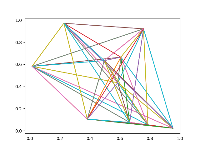
画出第一个例子的全部顶点和边。

{linenos

import matplotlib.pyplot as plt
points='0.607122 0.664447 0.953593 0.021519 0.757626 0.921024 0.586376 0.433565 0.786837 0.052959 0.016088 0.581436 0.496714 0.633571 0.227777 0.971433 0.665490 0.074331 0.383556 0.104392'
float_list = list(map(lambda x: float(x), points.split(' ')))

x,y = [],[]
for idx, p in enumerate(float_list):
  if idx % 2 == 0:
    x.append(p)
  else:
    y.append(p)

for i in range(0, len(x)):
  for j in range(0, len(x)):
    if i == j:
      continue
    plt.plot((x[i],x[j]),(y[i],y[j]))

plt.show()

全连接的图

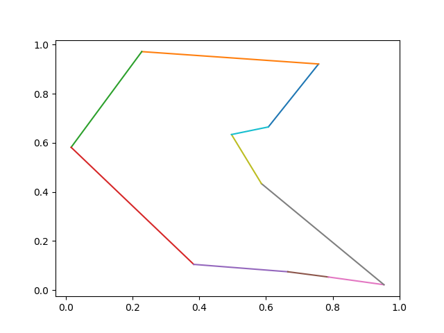
这个例子的最短TSP旅程为 \[ 1 \rightarrow 3 \rightarrow 8 \rightarrow 6 \rightarrow 10 \rightarrow 9 \rightarrow 5 \rightarrow 2 \rightarrow 4 \rightarrow 7 \rightarrow 1 \]

{linenos

tour_str = '1 3 8 6 10 9 5 2 4 7 1'
tour = list(map(lambda x: int(x), tour_str.split(' ')))

for i in range(0, len(tour)-1):
  p1 = tour[i] - 1
  p2 = tour[i + 1] - 1
  plt.plot((x[p1],x[p2]),(y[p1],y[p2]))
plt.show()

最短路径

PTR_NET TSP 的Python代码

初始化Init Graph Edges

在之前的自顶向下的递归版本中，需要做一些改动。首先，是图的初始化，我们依然延续之前的邻接矩阵来表示，由于这次的图是无向图，对于任意两个顶点，需要初始化双向的边。

{linenos

g: Graph = Graph(N)
for v in range(N):
	for u in range(N):
		diff_x = coordinates[v][0] - coordinates[u][0]
		diff_y = coordinates[v][1] - coordinates[u][1]
		dist: float = math.sqrt(diff_x * diff_x + diff_y * diff_y)
		g.setDist(u, v, dist)
		g.setDist(v, u, dist)

辅助变量记录父节点

另一大改动是需要在遍历过程中保存的顶点关联信息，以便在最终找到最短路径值时可以回溯对应的完整路径。在下面代码中，使用parent[bitstate][v] 来保存此状态下最小路径对应的顶点u。

{linenos

ret: float = FLOAT_INF
u_min: int = -1
	for u in range(self.g.v_num):
		if (state & (1 << u)) == 0:
			s: float = self._recurse(u, state | 1 << u)
				if s + edges[v][u] < ret:
					ret = s + edges[v][u]
					u_min = u
	dp[state][v] = ret
	self.parent[state][v] = u_min

当最终最短行程确定后，根据parent的信息可以按图索骥找到完整的行程顶点信息。

{linenos

def _form_tour(self):
	self.tour = [0]
	bit = 0
	v = 0
	for _ in range(self.g.v_num - 1):
		v = self.parent[bit][v]
		self.tour.append(v)
		bit = bit | (1 << v)
	self.tour.append(0)

需要注意的是，有可能存在多个最短行程，它们的距离值是一致的。这种情况下，代码输出的最短路径可能和数据集output后行程路径不一致，但是的两者的总距离是一致的。下面的代码验证了这一点。

{linenos

tsp: TSPSolver = TSPSolver(g)
tsp.solve()

output_dist: float = 0.0
output_tour = list(map(lambda x: int(x) - 1, output.split(' ')))
for v in range(1, len(output_tour)):
	pre_v = output_tour[v-1]
	curr_v = output_tour[v]
	diff_x = coordinates[pre_v][0] - coordinates[curr_v][0]
	diff_y = coordinates[pre_v][1] - coordinates[curr_v][1]
	dist: float = math.sqrt(diff_x * diff_x + diff_y * diff_y)
	output_dist += dist

	passed = abs(tsp.dist - output_dist) < 10e-5
	if passed:
		print(f'passed dist={tsp.tour}')
	else:
		print(f'Min Tour Distance = {output_dist}, Computed Tour Distance = {tsp.dist}, Expected Tour = {output_tour}, Result = {tsp.tour}')

本文所有代码在 github/MyEncyclopedia tsp/alg_plane 中。